ALGEBRA • INTERVALS • CALCULUS
Evaluate a piecewise function, one condition at a time
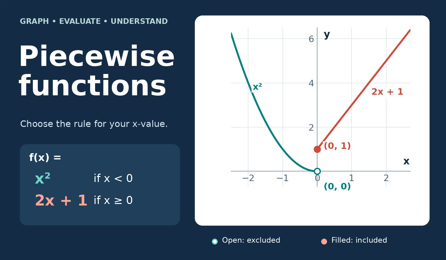
A piecewise function gives different rules for different inputs. To find f(a), first decide which condition includes a, then substitute a into that rule. For example, if f(x) = x² when x < 0 and f(x) = 2x + 1 when x ≥ 0, then f(−2) = 4, f(0) = 1 and f(2) = 5. The boundary belongs to the second piece because ≥ includes equality.
This calculator keeps your pieces visible, checks the conditions at your chosen x-value, and shows the selected expression and numerical result. It flags gaps, overlapping conditions and invalid expressions instead of silently selecting the first matching row. The lesson below explains domains, graphs, continuity, equations and calculus, with worked examples and practice answers.
Define your piecewise function
Enter a formula and a condition for each piece. Use Between for a finite interval and choose whether its endpoints are included. Use x = for a single input. Start by testing the default example at −2, 0 and 2.
Expression syntax and calculator limits
Write powers with ^, multiplication with *, and division with /. Parentheses group operations. Both 2*x and 2x are supported, as are 2(x+1) and x(x+1). Use − as an ordinary minus sign when writing by hand; in the input you can type the keyboard minus. −x² means −(x²), while (−x)² squares the negative input. Powers associate to the right: 2^3^2 means 2^(3^2). Multiplication, including implicit multiplication, and division have equal precedence and are evaluated left to right; use parentheses to make your intended grouping explicit.
Supported functions are sqrt, abs, sin, cos, tan, exp, ln, log, log10, floor and ceil. Functions require parentheses. Trigonometric angles are in radians; ln and log mean the natural logarithm, while log10 is base ten. pi and e are constants. Scientific notation such as 1e-8 is supported. Negative-base fractional powers and 0^0 are unsupported. For a negative cube root such as the cube root of −8, enter -(8^(1/3)) instead of (-8)^(1/3).
Inputs and results use approximate finite real-number arithmetic, not exact symbolic algebra. Detectable overflow and underflow are reported; cancellation and rounding can still affect results. The tool allows at most 30 pieces. Each expression is limited to 1,000 characters and 300 input tokens; deeply nested expressions are also rejected. x-values and bounds must be finite decimal or scientific-notation numbers. Comparisons use the stored numbers without an extra tolerance, so extremely close boundaries can round to the same value. The tool checks the supplied x, not the entire real line: a successful evaluation does not prove that all intervals are consistent, the function is continuous, or a graph has no hidden gaps. It does not automatically graph, differentiate, integrate or solve equations. These topics are taught below. To avoid silently choosing a rule, the tool flags every overlap at the entered x, even when the formulas happen to agree there.
Notation, intervals and the actual domain
Read a piecewise definition as a list of “formula, if condition” pairs. The condition chooses the rule; it is not another expression to add to the answer. In a textbook, the pairs usually sit beside one large brace. The same information can be written accessibly as a table:
| Formula for f(x) | Condition | Interval |
|---|---|---|
| x² | x < 0 | (−∞, 0) |
| 2x + 1 | 0 ≤ x < 3 | [0, 3) |
| 10 | x ≥ 3 | [3, ∞) |
A round bracket excludes an endpoint; a square bracket includes it. Infinity is not a real endpoint, so interval notation uses a round bracket at ±∞. For the middle piece, Between with “Lower only [)” represents 0 ≤ x < 3. At x = 3, use the third row, giving f(3) = 10, not 7.
A function need not be defined for every real number. A gap can be intentional. If the only conditions are x < 0 and x > 2, then [0, 2] is outside the stated domain. Do not fill a gap by extending a formula unless the definition tells you to. Also intersect each interval with its expression's real domain. A piece sqrt(x) for x < 2 allows 0 ≤ x < 2, not all x below 2. A piece 1/(x−1) cannot accept x = 1.
The defining requirement is one output for each input in the domain. Non-overlapping conditions are the clearest way to achieve that. Overlap is not automatically a mathematical contradiction: x² for x ≤ 0 and 0 for x ≥ 0 agree at x = 0. But x² for x ≤ 0 and 1 for x ≥ 0 assign two different values there and do not define a single-valued function. This calculator deliberately asks you to resolve overlapping rows; it does not try to prove equivalence.
If inequalities are the sticking point, revisit the negative-numbers lesson and check each boundary on a number line before evaluating.
Worked examples: select, substitute, check
1. Three intervals, three evaluations
Let f(x) = x + 3 for x < 1, x² for 1 ≤ x < 4, and 2x − 1 for x ≥ 4. The middle row uses Between, lower bound 1, upper bound 4 and “Lower only [)”.
- For f(0), the condition 0 < 1 is true. Use x + 3: 0 + 3 = 3.
- For f(2), 1 ≤ 2 < 4 is true. Use x²: 2² = 4.
- For f(4), the middle condition excludes 4. Use 2x − 1: 2(4) − 1 = 7.
Notice that f(1) = 1, even though substituting 1 into the first formula would give 4. A formula outside its specified interval does not give the function value.
2. Absolute value as two rules
For f(x) = |x|, use −x when x < 0 and x when x ≥ 0. Then f(−5) = −(−5) = 5, f(0) = 0 and f(3) = 3. The negative branch reverses the sign of a negative input; it does not make the output negative. You can enter this as two rows or use abs(x) in a single appropriate interval. See the absolute-value calculator for further practice.
3. A hypothetical progressive charge
These invented rates illustrate progressive brackets; they are not any country's current tax rules. Let income x be measured in dollars, x ≥ 0. Define T(x) as 0.10x for 0 ≤ x ≤ 10,000; 1000 + 0.15(x−10000) for 10,000 < x ≤ 40,000; and 5500 + 0.25(x−40000) for x > 40,000.
At $25,000, the second row applies: T(25000) = 1000 + 0.15(15000) = $3,250. At $50,000, the third row gives 5500 + 0.25(10000) = $8,000. The higher rate applies only to the amount above the threshold. Charging 25% of the whole $50,000 would give $12,500 and would describe a different model. At $40,000, the middle formula gives $5,500, matching the third branch's limiting value.
4. Solve an equation and reject out-of-interval answers
Solve f(x) = 5 where f(x) = x + 2 for x < 3 and x² − 4 for x ≥ 3. From the first rule, x + 2 = 5 gives x = 3, but 3 < 3 is false, so reject it in that branch. From the second, x² − 4 = 5 gives x = ±3. Only x = 3 satisfies x ≥ 3. The complete solution is therefore x = 3. Test the candidate in the original piecewise definition, not only in the equation you rearranged.
5. A branch with a hole in its expression
Let h(x) = (x²−1)/(x−1) when x ≠ 1, and h(1) = 5. In this tool, represent x ≠ 1 using separate x < 1 and x > 1 rows, then add an equality row at 1 with expression 5. For x ≠ 1, cancelling x−1 gives h(x) = x + 1. Hence h(0) = 1, h(2) = 3 and values near 1 approach 2. But h(1) remains 5. Cancellation does not change the separately defined value at the excluded input.
6. Find a constant for continuity
Let p(x) = x² for x < 2 and p(x) = kx + 1 for x ≥ 2. The left-hand limit is 4; the right-hand limit and p(2) are 2k + 1. Set 4 = 2k + 1, giving k = 3/2. This makes p continuous at 2. It does not make it differentiable there: the left slope is 2(2) = 4, while the right slope is 3/2.
Graph each piece only on its own interval
Start with the boundaries, then sketch each formula over its allowed x-values. At a finite boundary, an open circle excludes that point from that branch; a filled circle includes it, provided the expression has a defined value there. A formula with a vertical asymptote does not acquire a finite endpoint circle just because its interval ends.

For Example 1, the first branch approaches (1, 4), which is open. The second starts at the filled point (1, 1), approaches the open point (4, 16), and the third starts at the filled point (4, 7). These are jumps, not diagonal lines connecting the pieces. The function has exactly one y-value at each real x despite the two jumps. Two filled markers drawn at the same coordinate are redundant; two different filled y-values at the same x would violate the function rule.
Use a table of test inputs around every boundary: just below, exactly at, and just above. Test a point inside each interval too. Sampling helps find mistakes, but cannot prove global continuity or detect every narrow gap.
Continuity is about limits as well as the point value
At an interior boundary c, compare three things: the value approached from the left, the value approached from the right, and the defined value f(c). For ordinary two-sided continuity, both one-sided limits must exist as the same finite number and equal f(c). At an endpoint of a domain interval, use the appropriate one-sided condition.
Substitution is a method, not the definition of a limit. With polynomial branches such as x² and 2x, you can substitute c to get their one-sided limits. A quotient like (x²−1)/(x−1) needs simplification or another valid limit argument at c = 1. Direct substitution gives 0/0, not a numerical limit.

Example A: continuous but with unequal slopes
Take f(x) = x² for x < 2, 4 for x = 2, and 2x for x > 2. The left limit is 4, the right limit is 4 and f(2) = 4. It is continuous at 2. Its one-sided slopes are 4 and 2, so it is not differentiable there.
Example B: a jump
Take g(x) = x + 1 for x < 1 and 3 for x ≥ 1. The left limit is 2; the right limit and g(1) are 3. Since 2 ≠ 3, the two-sided limit does not exist and the function is discontinuous at 1. A filled endpoint on one piece does not repair a mismatch between the limits.
In Example 5, both limits equal 2 while h(1) = 5. That is a removable discontinuity: changing the value at 1 to 2 makes the function continuous. By contrast, changing just the boundary value cannot remove Example B's jump.
Derivatives, integrals and extensions
Inside a piece's open interval, differentiate its formula wherever that derivative exists. At a joining point c, check continuity and compare the one-sided limits of the difference quotient (f(c+h)−f(c))/h as h approaches 0 from the left and right. Both derivative limits must exist as the same finite number. Equal-looking formulas or a smooth-looking low-resolution graph are not proofs. For |x|, the left derivative at 0 is −1 and the right derivative is 1: the function is continuous but has a corner and no derivative at 0.
For a definite integral of an integrable piecewise function, split the integration interval at the boundaries and add the integrals. For example, let q(x) = x on 0 ≤ x < 2 and q(x) = 4 on 2 ≤ x ≤ 3. The integral from 0 to 3 is the triangle area ½ × 2 × 2 plus the rectangle area 1 × 4, giving 6. A single endpoint's assigned value does not change this integral. If a branch becomes unbounded at a split, examine the resulting improper integrals rather than assuming a finite answer.
Composition: evaluate the inside function first. If f(x) is Example 2's absolute value and g(x) = x−3, then (f∘g)(1) = f(−2) = 2. The branch of f is selected using −2, not the original input 1.
Piecewise sequences: an index can choose the rule. If an = n² for even positive n and 2n for odd positive n, the first six terms are 2, 4, 6, 16, 10, 36. These are parity conditions, which are taught here but are not a separate condition mode in the interval calculator.
Periodic signals: square waves are a common piecewise model in Fourier analysis. For piecewise-smooth periodic functions, the Fourier series approaches the function at continuity points and the midpoint of the two one-sided limits at a jump. It need not reproduce a separately chosen boundary value there. The calculator evaluates individual expressions, not a Fourier series.
Special functions and real-world models
| Function | Rules or interpretation | Check |
|---|---|---|
| Absolute value |x| | −x for x < 0; x for x ≥ 0 | |−2.3| = 2.3 |
| Sign function | −1 for x < 0; 0 for x = 0; 1 for x > 0 | sgn(0) = 0 |
| Step function | Here choose 0 for x < 0 and 1 for x ≥ 0 | The value at 0 is a convention; state it |
| Floor | Largest integer ≤ x; n on [n, n+1) | floor(−2.3) = −3 |
| Ceiling | Smallest integer ≥ x; n on (n−1, n] | ceil(−2.3) = −2 |
Shipping, postal rates, parking fees, sales commission and utility charges often have thresholds. Read whether a new rate applies to the whole amount or only the excess: these create different formulas. Daily caps add a constant final piece. Deductible-and-reimbursement models need clear coverage and cap assumptions; investment-rate examples need a stated balance rule and time period. These are mathematical modeling patterns, not tax, insurance or investment advice.
In physics, motion can use separate acceleration or velocity formulas over time intervals. Keep time and distance units consistent. A simple on/off temperature rule is piecewise, but thermostat hysteresis also depends on the previous on/off state. Two temperature thresholds alone do not define the output as a function of temperature only; include state in the model.
Common mistakes to catch
- Using every formula: evaluate the applicable rule, not the sum of all rules.
- Forgetting equality: x < 4 excludes 4; x ≤ 4 includes it. Check the exact boundary separately.
- Assuming a gap is an error: it is an error only if the intended domain includes those missing inputs.
- Ignoring formula restrictions: an interval cannot make division by zero or a negative real square root valid.
- Trusting the first matching row: overlapping rules need agreement wherever both apply. Resolve the definition before using the calculator.
- Confusing continuity with differentiability: a joined graph can still have a corner.
- Keeping every algebraic solution: each candidate must satisfy the condition of the branch that produced it.
- Reading a rounded zero as proof: use scientific notation and check approximate arithmetic when values are very small.
Try it yourself
Use the definition in each question. Decide the piece before doing the arithmetic, then open the answer to check your reasoning.
1. For Example 1, find f(−2), f(1) and f(5)
f(−2) = −2 + 3 = 1; f(1) = 1² = 1; f(5) = 2(5) − 1 = 9.
2. The rules are x² for x < 0 and x + 2 for x > 0. What is f(0)?
Undefined. Neither condition includes 0. If the intended domain is all reals, add a value at 0; otherwise the excluded point can be intentional.
3. The rules are x + 1 for x ≤ 2 and 7 for x ≥ 2. Is this a function at 2?
No. Both conditions apply, giving 3 and 7. There is no unique output at 2.
4. For sqrt(x−1) on 0 ≤ x < 5, what is the real domain?
[1, 5). The square root requires x−1 ≥ 0, so intersect x ≥ 1 with the stated interval.
5. Find k if x + 4 for x < 2 and kx for x ≥ 2 must join continuously
The left limit is 2 + 4 = 6. Set 2k = 6, so k = 3. The slopes still differ: 1 versus 3.
6. Evaluate floor(−1.2) and ceil(−1.2)
−2 and −1, respectively. Floor moves toward negative infinity; ceiling toward positive infinity.
7. Solve f(x) = 4 for f(x) = x² when x < 0 and x + 1 when x ≥ 0
The first branch gives ±2, but only −2 is negative. The second gives 3, which is nonnegative. The solutions are x = −2 and x = 3.
8. A speed is 3 m/s for 0 ≤ t < 2 s and 5 m/s for 2 ≤ t ≤ 4 s. Find distance
Add the two rectangle areas: 3 × 2 + 5 × 2 = 16 m. This assumes the stated speeds are nonnegative, so the speed integral is distance.
Frequently asked questions
What is a piecewise function?
A function defined by different formulas on specified parts of its domain. Each permitted input must have one output. Piecewise does not mean discontinuous: |x| is a continuous example.
How do you evaluate a piecewise function?
Check which condition includes the input, select that formula, substitute and calculate. For x + 1 when x < 2 and x² when x ≥ 2, f(3) = 3² = 9.
What is the difference between strict and non-strict inequalities?
< and > exclude equality; ≤ and ≥ include it. Between can include neither endpoint, the lower only, the upper only or both. Use disjoint conditions when possible. Mathematical overlap is harmless only if it never gives conflicting or undefined values.
Are piecewise functions continuous?
Some are. The rules x for x < 1 and x² for x ≥ 1 join continuously at 1 because both one-sided limits and f(1) equal 1. The rules x for x < 1 and x + 1 for x ≥ 1 have a jump because their limits are 1 and 2.
How are piecewise functions used in real life?
They model changing rates, caps and thresholds in shipping, utility charges, motion and other settings. Specify the units, domain and assumptions. A system with memory, such as a hysteresis controller, also needs a state variable.
How do you find the domain of a piecewise function?
For each row, intersect the condition with the real domain of its formula, then take the union. Separately check that overlapping rows do not assign conflicting outputs. The result need not be all real numbers.
Can piecewise functions have more than two pieces?
Yes. For example, x³ for x < −1, x² for −1 ≤ x < 0, x for 0 ≤ x < 1 and sqrt(x) for x ≥ 1 has four pieces. A single-point equality row is also a valid piece.
How do you graph a piecewise function?
Sketch each formula only where its condition applies, mark finite included endpoints with filled circles and excluded endpoints with open circles, and check each boundary value. Do not connect a jump with an invented line segment.
Sources & References
These references support the definitions and methods. The worked examples, practice set, diagrams and calculator implementation on this page are independently prepared.
- OpenStax Precalculus 2e: Domain and Range — piecewise conditions, intervals and graphs.
- OpenStax Calculus Volume 1: Continuity — limits, point values and one-sided continuity.
- NIST Digital Library of Mathematical Functions: Mathematical Introduction — floor, ceiling and sign definitions.
- MIT OpenCourseWare: Fourier Series Introduction Continued (PDF) — square-wave series and convergence to the midpoint at a jump.
- MathWorks: Relay — state-dependent switching and hysteresis.