STATISTICS PRACTICE • KS3 TO GCSE
Find statistics worksheets by topic, learn the method, then check your answers. This collection keeps all 38 original worksheet activities, with PDF and editable Word versions from Dr Austin Maths, plus original worked examples and a new 10-question practice sheet.
Browse the 38 worksheet activities Try the original practice questions
The linked worksheets belong to Dr Austin Maths. The explanations, diagrams and original practice on this page are by HeLovesMath. Download links and full source credit are together in Sources & References.
Which statistics worksheet should I use?
Choose one skill you can explain, not simply a sheet with a familiar title. If you are revising for an exam, use your own course specification: these topics span different ages and tiers, and this collection is not a complete examination syllabus.
| Your next skill | Start here | Ready to move on when… |
|---|---|---|
| Summarise a short list | Averages and range | You order the data, count every value and explain what each statistic tells you. |
| Handle repeated values | Frequency tables and combined means | You can recover totals from frequencies instead of averaging the row labels. |
| Represent data clearly | Bar charts, pie charts and frequency polygons | You choose an appropriate graph, label its axes and use a consistent scale. |
| Estimate from grouped data | Grouped means | You use class midpoints and say why the answer is an estimate. |
| Study distributions in more detail | Quartiles, cumulative frequency and histograms | You distinguish cumulative totals, density and frequency. |
Tier guide: averages, range, frequency tables, bar charts and pie charts provide core practice. AQA GCSE Mathematics places histograms, cumulative-frequency graphs, quartiles and interquartile range in Higher-tier content. Other qualifications organise their content differently; a worksheet title alone does not establish its tier.
For a short revision session, read one worked example, attempt a matching sheet without its answers, then correct each error in words. “I divided by the number of rows instead of the total frequency” gives you a useful next step; copying the answer does not.
Mean, median, mode and range: one data set, four questions
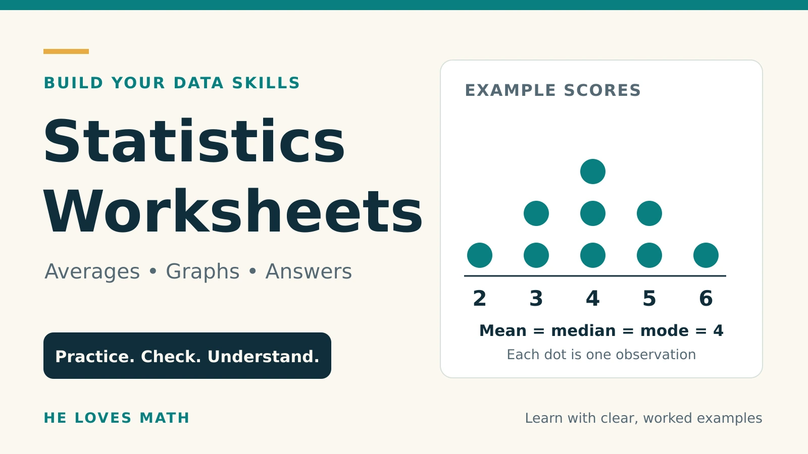
The mean, median and mode describe a centre or a common value. The range describes spread. They are not interchangeable, and a sensible comparison usually discusses both a typical value and variability.
Worked example: reading times
Six pupils spend 4, 7, 7, 8, 10 and 12 minutes reading.
- Mean: add all six times, then divide by six. (4 + 7 + 7 + 8 + 10 + 12) ÷ 6 = 48 ÷ 6 = 8 minutes.
- Median: the list is already in order. With six values, average the third and fourth: (7 + 8) ÷ 2 = 7.5 minutes.
- Mode: 7 occurs twice, more often than any other value, so the mode is 7 minutes.
- Range: largest minus smallest, 12 − 4 = 8 minutes.
The median can lie between two observed values. It does not need to appear in the list. A data set can also have more than one mode: 2, 2, 5, 5, 9 has modes 2 and 5. In the usual school convention, a list in which every value occurs once is described as having no mode.
What changes when there is an extreme value?
Replace 12 with 42 in the reading-time example. The total rises from 48 to 78, so the mean becomes 78 ÷ 6 = 13 minutes. The median remains 7.5 minutes and the mode remains 7 minutes. The range becomes 42 − 4 = 38 minutes. This shows why one unusually large observation can move the mean and range substantially.
Do not automatically discard an extreme value. First check whether it is a recording error or a genuine observation. If it is genuine, explain its effect and choose the summary that suits the question. For categorical data such as favourite colours, a mode can be meaningful; a numerical mean cannot.
Common traps: finding the middle of an unordered list; dividing by the number of different values; reporting the highest frequency as the mode; adding the largest and smallest values when finding the range.
Frequency tables and combined means
A frequency tells you how many observations have a particular value. If a score of 3 occurs four times, those observations contribute 3 × 4 = 12 to the total score.
| Books, x | Frequency, f | x × f | Cumulative frequency |
|---|---|---|---|
| 0 | 2 | 0 | 2 |
| 1 | 3 | 3 | 5 |
| 2 | 4 | 8 | 9 |
| 3 | 1 | 3 | 10 |
| Total | 10 | 14 | — |
Mean = total of x × f ÷ total frequency = 14 ÷ 10 = 1.4 books. The fifth observation is 1 and the sixth is 2, so the median is 1.5 books. The mode is 2 books because that value has the largest frequency, 4. The range is 3 − 0 = 3 books.
A mean of 1.4 books is a summary across pupils; it does not claim that any pupil read exactly 1.4 books. Check that the mean lies between the smallest and largest values.
Worked example: combining two means
A group of 12 learners has mean score 6. A second group of 18 has mean score 8. The groups are separate and use the same scoring scale.
- Recover the totals: 12 × 6 = 72 and 18 × 8 = 144.
- Add the scores and group sizes: total score 216, total learners 30.
- Combined mean = 216 ÷ 30 = 7.2.
The simple average (6 + 8) ÷ 2 = 7 gives equal weight to unequal groups and is wrong here. The larger group pulls the combined mean closer to 8.
If the published group means were rounded, a combined mean calculated from them may also be approximate. Do not give extra decimal places as though the original information were exact.
Choose the graph to match the question
| Graph | Use it for | Check before drawing |
|---|---|---|
| Bar chart | Comparing category frequencies or discrete values | Equal-width bars, gaps and a labelled frequency scale. Comparative bars need a key; stacked bars show components of totals. |
| Pie chart | Showing how categories divide one whole | All categories must cover the whole without overlap. Sector angles add to 360°. |
| Line graph | Following a quantity over time | Keep times in order and space them according to the time scale. |
| Frequency polygon | Comparing the shape of grouped distributions with equal class widths | For equal-width classes, plot class midpoint against frequency, then join neighbouring points. Midpoints are not class boundaries. |
| Histogram | Showing grouped continuous data | With unequal class widths, use frequency density so area represents frequency. |
| Cumulative-frequency graph | Estimating medians, quartiles and counts below a boundary | Plot running totals at upper class boundaries; a cumulative total cannot decrease. |
Worked example: a pie-chart sector
In a survey of 30 pupils, 12 choose walking as their main journey to school. The sector angle is (12 ÷ 30) × 360° = 144°. Walking represents 40% of this group.
Use the survey total, 30, as the denominator. A 144° sector does not mean 144 pupils. Conversely, if a 90° sector represents 8 pupils, the whole group contains 8 × (360 ÷ 90) = 32 pupils.
When comparing two groups, raw frequencies may be misleading if the group sizes differ. For example, 10 out of 20 is 50%, whereas 15 out of 50 is 30%. The second count is larger but the first proportion is larger.
Scatter graphs: association is not a cause
A scatter graph uses paired measurements, such as each pupil’s study time and test score. An upward pattern suggests positive correlation. It does not prove that one variable causes the other: previous knowledge, other study activities or sampling choices could influence both. Predictions far beyond the observed values are particularly uncertain.
Grouped data: estimated means and histogram density
Grouping hides individual values. A class such as 10 ≤ t < 20 includes 10 minutes but excludes 20 minutes; the next class starts at 20. Keep boundaries consistent so every observation belongs to exactly one class.
| Time t (minutes) | Frequency | Midpoint | Width | Density |
|---|---|---|---|---|
| 0 ≤ t < 10 | 8 | 5 | 10 | 0.8 |
| 10 ≤ t < 20 | 12 | 15 | 10 | 1.2 |
| 20 ≤ t < 40 | 20 | 30 | 20 | 1.0 |
Estimated mean: use each midpoint as a representative journey time. The estimated total is 5 × 8 + 15 × 12 + 30 × 20 = 40 + 180 + 600 = 820 minutes. Divide by the total frequency: 820 ÷ 40 = 20.5 minutes.
This is an estimate because the exact times within each interval are unknown. Do not divide the estimated total of 820 by the three classes: the classes contain different numbers of people. Do not claim the estimate is the true mean.
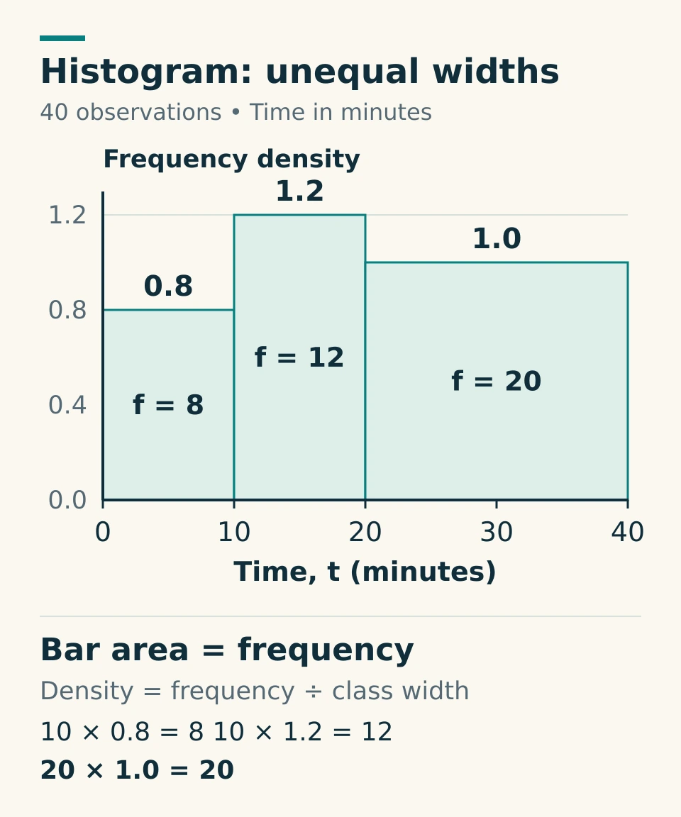
Frequency density = frequency ÷ class width. For the final class, 20 ÷ 20 = 1 person per minute on the density scale. Multiplying its width by its height gives 20 × 1 = 20 people. All three areas add to 40.
The height trap: the tallest bar, 10 ≤ t < 20, has the highest density, but the widest class, 20 ≤ t < 40, has the greatest frequency. Looking only at height loses the effect of class width. Read what the axis measures before using a histogram.
Cumulative frequency, median and quartiles
For the same journey-time data, the running totals are 8, 20 and 40. Plot the upper boundaries against these totals: (10, 8), (20, 20), (40, 40), starting at (0, 0). Cumulative frequency 20 at 20 minutes means 20 journeys are below 20 minutes under these class definitions.
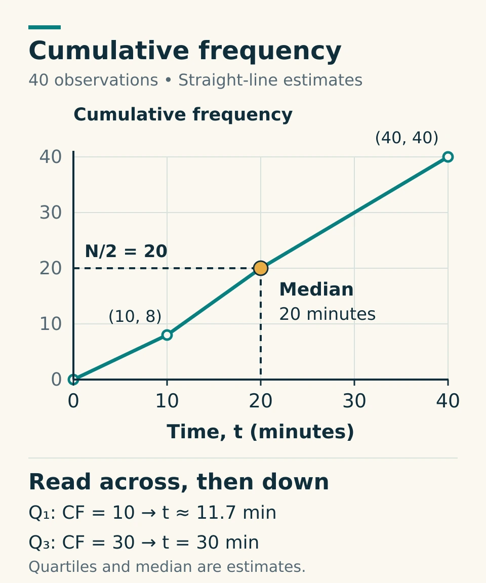
With N = 40 observations, read the lower quartile at N ÷ 4 = 10, the median at N ÷ 2 = 20, and the upper quartile at 3N ÷ 4 = 30 on the cumulative-frequency axis.
- Estimated median: 20 minutes.
- Estimated lower quartile Q1: 10 + [(10 − 8) ÷ 12] × 10 ≈ 11.7 minutes.
- Estimated upper quartile Q3: 20 + [(30 − 20) ÷ 20] × 20 = 30 minutes.
- Estimated interquartile range: Q3 − Q1 ≈ 18.3 minutes, using unrounded values before rounding the result.
The interpolation assumes observations are spread uniformly within each class. The grouped data do not reveal the exact raw-data median or quartiles. A hand-drawn curve may give slightly different estimates; use the method and accuracy required by your question.
Raw lists use a stated quartile convention
Different textbooks and software use different definitions of sample quartiles. In the original practice below, use this rule for a raw list: order the values, find the median, then find the median of each half; for an odd-sized list, leave out the central observation from both halves. Follow your exam board or teacher if a different convention is specified.
For 2, 4, 5, 7, 8, 10, 12, 16, the median is (7 + 8) ÷ 2 = 7.5, Q1 = (4 + 5) ÷ 2 = 4.5 and Q3 = (10 + 12) ÷ 2 = 11. The IQR is 11 − 4.5 = 6.5. The range, 16 − 2 = 14, uses the extremes instead.
To compare distributions, connect the statistics to the context. “Group A has a smaller median journey time and a smaller IQR, so its typical journey is shorter and its middle half is less spread out” is more informative than “A is better”.
Original statistics practice: 10 questions with worked answers
Attempt the questions before opening the solutions. Keep units in your working, state when an answer is estimated and use the raw-list quartile convention above. These are original HeLovesMath questions, separate from the linked Dr Austin Maths worksheets.
Download the practice sheet and answers (PDF)
1. Mean, median, modes and range
Eight scores are 6, 8, 3, 6, 10, 3, 9 and 7.
Find the mean, median, all modes and range.
Show worked answer 1
Ordered scores: 3, 3, 6, 6, 7, 8, 9, 10.
- Sum = 52, so mean = 52 / 8 = 6.5.
- There are eight scores. Median = (4th value + 5th value) / 2 = (6 + 7) / 2 = 6.5.
- Both 3 and 6 occur twice; every other value occurs once. The modes are 3 and 6.
- Range = 10 − 3 = 7.
2. An unusually long journey
Six journey times, in minutes, are 12, 13, 14, 14, 15 and 16.
(a) Find their mean and median. (b) Replace 16 with 76 and find the new mean and median. (c) Which average better describes the centre of the revised list, and why?
Show worked answer 2
Original total = 12 + 13 + 14 + 14 + 15 + 16 = 84 minutes.
- Original mean = 84 / 6 = 14 minutes.
- Original median = (14 + 14) / 2 = 14 minutes.
- Revised total = 84 − 16 + 76 = 144 minutes, so new mean = 144 / 6 = 24 minutes.
- The middle two values remain 14 and 14, so new median = 14 minutes.
- The median better represents the centre of these six revised times: five are between 12 and 15 minutes, while the unusually long journey pulls the mean upward. This does not prove that 76 is a recording error.
3. A discrete frequency table
Twenty-four players earned the following numbers of stars.
| Stars, x | 0 | 1 | 2 | 3 | 4 |
|---|---|---|---|---|---|
| Frequency, f | 3 | 6 | 8 | 5 | 2 |
Find the mean, median, mode and range of the numbers of stars.
Show worked answer 3
| x | f | fx | Cumulative frequency |
|---|---|---|---|
| 0 | 3 | 0 | 3 |
| 1 | 6 | 6 | 9 |
| 2 | 8 | 16 | 17 |
| 3 | 5 | 15 | 22 |
| 4 | 2 | 8 | 24 |
| Total | 24 | 45 | — |
- Mean = sum(fx) / sum(f) = 45 / 24 = 1.875 stars.
- Median positions are 12 and 13. Positions 10 through 17 all contain 2 stars, so median = (2 + 2) / 2 = 2 stars.
- Highest frequency is 8, attached to x = 2, so mode = 2 stars, not 8.
- Range = 4 − 0 = 4 stars.
4. Combining groups of unequal size
Group A has 12 players with a mean score of 18 points. Group B has 18 players with a mean score of 23 points. Each player belongs to exactly one group.
Find the mean score for all 30 players. Explain why (18 + 23) / 2 is not the correct method here.
Show worked answer 4
Group A total = 12 × 18 = 216 points. Group B total = 18 × 23 = 414 points.
Combined mean = (216 + 414) / (12 + 18) = 630 / 30 = 21 points.
(18 + 23) / 2 = 20.5 gives the two groups equal weight, even though their sizes differ. Weight each mean by its group size.
5. Estimating a mean from grouped data
Twenty delivery times are summarised below.
| Time, t (minutes) | Frequency |
|---|---|
| 0 ≤ t < 10 | 4 |
| 10 ≤ t < 20 | 8 |
| 20 ≤ t < 40 | 6 |
| 40 ≤ t < 60 | 2 |
Use class midpoints to estimate the mean delivery time. Explain why this is an estimate.
Show worked answer 5
| Time (minutes) | f | Midpoint, m | fm |
|---|---|---|---|
| 0 ≤ t < 10 | 4 | 5 | 20 |
| 10 ≤ t < 20 | 8 | 15 | 120 |
| 20 ≤ t < 40 | 6 | 30 | 180 |
| 40 ≤ t < 60 | 2 | 50 | 100 |
| Total | 20 | — | 420 |
Estimated mean = 420 / 20 = 21 minutes.
Only intervals are known; each midpoint represents the unknown times within its interval. Therefore 21 minutes is an estimate, not a mean recovered from the original observations.
6. Pie-chart sectors
Of 72 club members, 18 cycle to the club, 24 take the bus and 30 walk. Each member selects exactly one of these travel methods.
Calculate the angle of each sector in a pie chart, and check that the angles total 360°.
Show worked answer 6
Sector angle = category frequency / 72 × 360°.
- Cycle: 18 / 72 × 360° = 90°.
- Bus: 24 / 72 × 360° = 120°.
- Walk: 30 / 72 × 360° = 150°.
- Check: 90° + 120° + 150° = 360°.
7. Quartiles and interquartile range — Higher extension
The nine values are 13, 2, 9, 6, 20, 11, 8, 4 and 15.
For this question, order the values, exclude the overall median from both halves when there is an odd number of values, and take the median of each half as Q1 and Q3. This is the stated median-of-halves convention; other conventions can give different results.
Find the median, lower quartile Q1, upper quartile Q3 and interquartile range.
Show worked answer 7
Ordered values: 2, 4, 6, 8, 9, 11, 13, 15, 20.
- Median is the 5th value: 9.
- Exclude 9. Lower half: 2, 4, 6, 8. Q1 = (4 + 6) / 2 = 5.
- Upper half: 11, 13, 15, 20. Q3 = (13 + 15) / 2 = 14.
- IQR = Q3 − Q1 = 14 − 5 = 9.
These are the answers under the stated convention. For example, some interpolation conventions give Q1 = 6 and Q3 = 13 for this same list; that does not invalidate the explicitly chosen method.
8. Cumulative-frequency estimates — Higher extension
Forty waiting times have this cumulative-frequency table. The cumulative frequency gives the number of times at most the upper boundary.
| Upper boundary, t (minutes) | 0 | 10 | 20 | 30 | 40 | 50 |
|---|---|---|---|---|---|---|
| Cumulative frequency | 0 | 4 | 12 | 24 | 36 | 40 |
Plot these points with time on the horizontal axis and cumulative frequency on the vertical axis. For this question, join consecutive points with straight lines.
(a) Estimate Q1, the median and Q3. (b) Estimate the IQR. (c) Estimate the number of people who waited more than 35 minutes. Give the median to 1 decimal place. Use N/4, N/2 and 3N/4 on the cumulative-frequency axis. All readings are estimates of the original ungrouped data.
Show worked answer 8
N = 40, so read Q1 at cumulative frequency 10, the median at 20, and Q3 at 30. Plotting the supplied points and joining them linearly gives:
- Q1 is between (10, 4) and (20, 12). The required increase is 10 − 4 = 6 out of a total rise of 8: Q1 = 10 + (6 / 8) × 10 = 17.5 minutes.
- Median is between (20, 12) and (30, 24): median = 20 + ((20 − 12) / (24 − 12)) × 10 = 20 + 20/3 = 80/3 ≈ 26.7 minutes.
- Q3 is between (30, 24) and (40, 36): Q3 = 30 + ((30 − 24) / (36 − 24)) × 10 = 35 minutes.
- IQR ≈ 35 − 17.5 = 17.5 minutes.
- At 35 minutes, estimated cumulative frequency = 24 + (5 / 10) × 12 = 30. Estimated number waiting more than 35 minutes = 40 − 30 = 10 people.
All are estimates because individual waiting times inside each interval are unknown. A smooth curve instead of the specified straight segments could give slightly different readings.
9. Histogram with unequal class widths — Higher extension
The table describes a frequency-density histogram of completion times.
| Time, t (minutes) | Frequency | Frequency density |
|---|---|---|
| 0 ≤ t < 5 | 20 | ? |
| 5 ≤ t < 15 | 30 | ? |
| 15 ≤ t < 35 | 40 | ? |
| 35 ≤ t < 45 | ? | 1.5 |
(a) Complete the table. (b) Find the total frequency. (c) Identify the tallest bar and the class with the greatest frequency. Explain why they differ. (d) Assuming an even spread of times within each class, estimate how many times satisfy 10 ≤ t < 25.
Show worked answer 9
Class width = upper boundary − lower boundary. Density = frequency / class width.
| Time (minutes) | Width | Frequency | Density |
|---|---|---|---|
| 0 ≤ t < 5 | 5 | 20 | 20 / 5 = 4 |
| 5 ≤ t < 15 | 10 | 30 | 30 / 10 = 3 |
| 15 ≤ t < 35 | 20 | 40 | 40 / 20 = 2 |
| 35 ≤ t < 45 | 10 | 10 × 1.5 = 15 | 1.5 |
- Total frequency = 20 + 30 + 40 + 15 = 105.
- Tallest bar: 0 ≤ t < 5, with density 4.
- Greatest frequency: 15 ≤ t < 35, with 40 observations. It is wider, so its larger area can occur despite its smaller height.
- From 10 to 15 minutes: half of the second class, giving (5 / 10) × 30 = 15.
- From 15 to 25 minutes: half of the third class, giving (10 / 20) × 40 = 20.
- Estimated count for 10 ≤ t < 25 = 15 + 20 = 35.
The last calculation requires the stated even-spread assumption; the table alone does not determine the exact count.
10. Correlation, causation and prediction
A scatter graph of a park shop’s daily ice-cream sales and daily sunhat sales shows that days with more ice creams sold tend to have more sunhats sold. The observed ice-cream sales range from 40 to 180 per day.
(a) Name the direction of correlation. (b) Is the claim “selling more ice creams causes more sunhats to be sold” justified by this graph alone? Explain. (c) Suggest a possible third variable. (d) Explain why using a line of best fit to predict sunhat sales on a day when 300 ice creams are sold would be uncertain.
Show worked answer 10
(a) Positive correlation. The wording does not supply enough detail to grade its strength.
(b) No. An association between the sales totals does not establish that one causes the other.
(c) Weather/temperature is a plausible third variable: hotter, sunnier days might increase demand for both. Park attendance is another reasonable answer. Neither explanation is proved by the graph.
(d) 300 is outside the observed range of 40–180, so this is extrapolation. The observed relationship may not continue that far, making the prediction less reliable.
Check your work before moving on
- Totals: frequencies sum to the sample size; pie angles sum to 360°; the last cumulative total matches the number of observations.
- Location: the mean and median are between the smallest and largest values. Check whether you reported a data value or a frequency.
- Units: an average journey time is in minutes; a histogram density is in people per minute, not simply people.
- Precision: keep unrounded calculations until the final answer. Grouped-data estimates cannot restore missing individual measurements.
- Interpretation: discuss centre and spread, and distinguish association from causation.
For related practice, use the probability worksheet collection for chance and sample spaces, or the algebra worksheets to strengthen the equation skills used when finding a missing frequency or unknown value.
Sources & References
Worksheet downloads: all 38 original activities
These third-party worksheets are created and hosted by Dr Austin Maths. We link to the original files rather than rehosting them. Please respect the creator’s terms. “PDF” opens the question sheet; “Answers” opens the linked answer sheet; “Editable Word” opens a DOCX file. The Wordsearch versus Sudoku activity has no separate answer-file link in the original collection.
All 113 original file links were checked on 4 October 2026. File availability can change. If a file stops opening, visit the creator’s statistics collection above. Link checks do not mean every third-party question or answer has been independently re-marked.
Averages and range
Core practice: build fluency with short lists, then explain your choices.
- Mode, Median and Range Practice Strips
- Mode, Median and Range Match-Up
- Mean Practice Strips
- Mean Crack the Code
- Averages and Range Practice Strips
- Averages and Range Fill In The Blanks
- Averages and Range Odd One Out
- Averages and Range True or False
- Averages and Range Maths Challenge Questions
- Averages and Range Revision Practice Grid
Frequency tables and combined means
Recover totals, use frequencies and combine unequal groups carefully.
- Combining Means Fill in the Blanks
- More Combining Means Fill in the Blanks
- Combining Means Practice Strips
- Averages from a Frequency Table Practice Strips
- Mean from a Frequency Table Fill In The Blanks
- Mean from a Table Crack the Code
Estimated means from grouped tables
Use midpoints and label the calculated mean as an estimate.
- Mean from a Grouped Frequency Table Practice Strips
- Mean from a Grouped Frequency Table Fill In The Blanks
Median and quartiles
Quartiles are a Higher extension in AQA GCSE Mathematics. Check the convention required.
- Median and Quartiles Practice Strips
- Median and Quartiles Fill In The Blanks
Bar charts, pie charts and frequency polygons
Choose the representation that matches the variable and the question.
- Drawing Comparative Bar Charts Practice Grid
- Drawing Composite Bar Charts Practice Grid
- Drawing Pie Charts Practice Grid
- Pie Charts Fill in the Blanks
- Plotting Frequency Polygons Practice Grid
- Plotting Line Graphs Practice Grid
- Representing Statistical Data Revision Practice Grid
Cumulative frequency
Higher extension: running totals, graph readings and quartile estimates.
- Cumulative Frequency Graphs – Wordsearch versus Sudoku Activity
- Plotting Cumulative Frequency Graphs Practice Grid
- Reading Cumulative Frequency Graphs Practice Grid
- Finding Frequencies from Cumulative Frequency Graphs Practice Grid
- Cumulative Frequency Graphs Practice Grid
Histograms
Higher extension: use density for unequal class widths and interpret area.
- Plotting Histograms Practice Grid
- Plotting Incomplete Histograms Practice Grid
- Histograms Match-Up
- Interpreting Histograms Practice Grid
- Finding the Median from a Histogram Practice Grid
- Histograms Practice Grid
References for the original explanations
- AQA GCSE Mathematics 8300: statistics content and tier requirements.
- AQA: Exploring common misunderstandings in GCSE Maths, including grouped mean estimates.
- NIST/SEMATECH: measures of location, for mean, median and mode.
- NIST/SEMATECH: percentiles, explaining differing sample-quantile methods.
- WJEC: histograms, including frequency density and within-class estimation.