
AQA · A-level Mathematics · 7357
Download AQA A-level Mathematics 7357 past papers and matching mark schemes, organised by series and paper. Use the revision method, original worked examples and eight-question diagnostic below to find the next skill to practise.
Archive coverage: June 2018, June 2019, November 2020, November 2021 and June 2022, plus specimen set 1 and commentary. All 37 original resource links are retained. This is a useful older-paper collection, not a claim to contain every released series.
How the three 7357 papers fit together
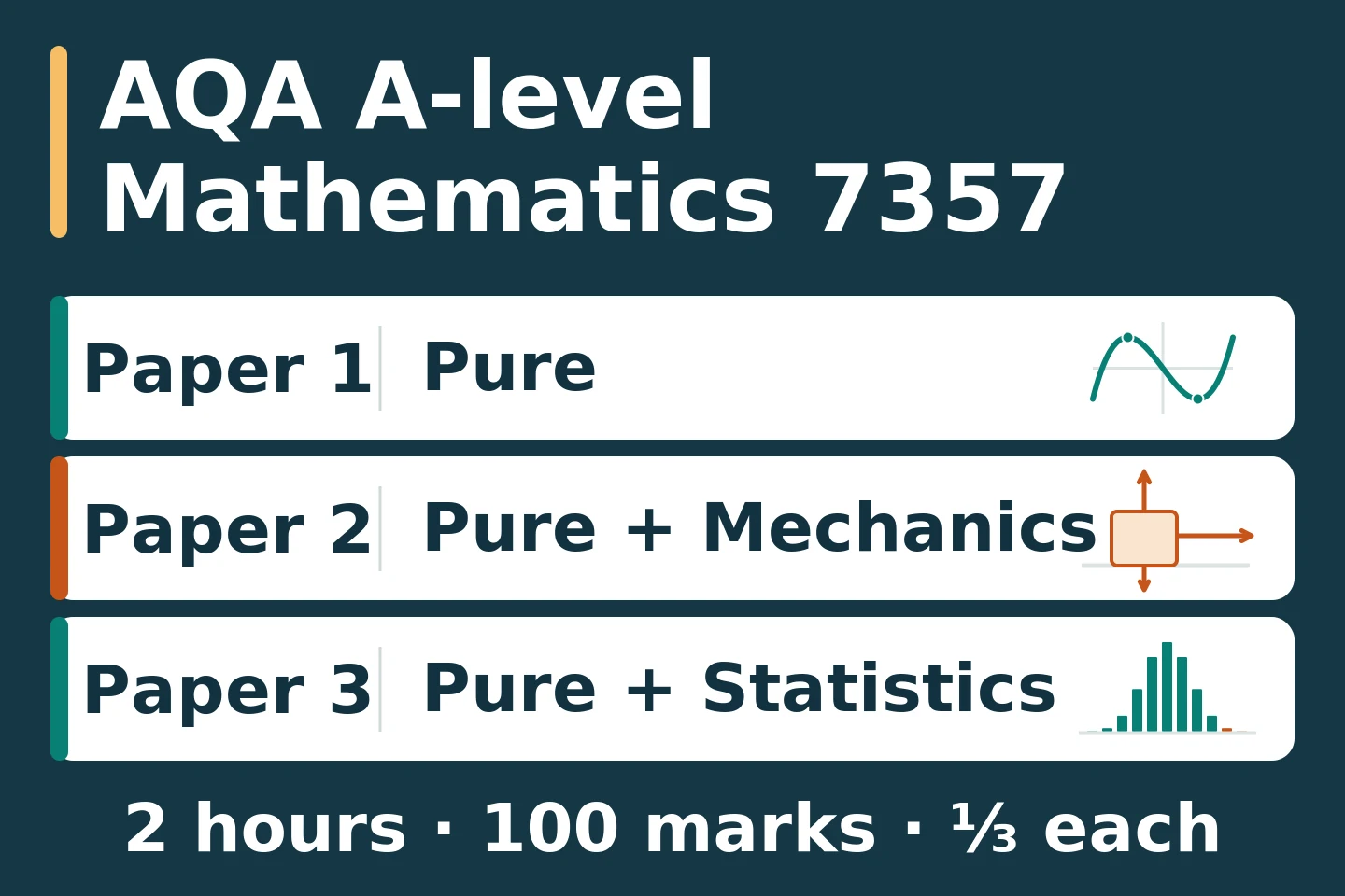
AQA 7357 is linear: its three examinations are taken at the end of the course. Each paper lasts 2 hours, carries 100 marks and contributes one-third of the A-level. Pure mathematics is assessed across the set, so do not prepare mechanics or statistics in isolation.
Paper 1 · 7357/1
Pure mathematics, topics A–I
Proof, algebra, coordinate geometry, sequences, trigonometry, exponentials and logarithms, differentiation, integration and numerical methods.
Paper 2 · 7357/2
Pure mathematics and mechanics
Paper 1 content plus vectors (J), quantities and units, kinematics, forces and Newton’s laws, and moments (P–S).
Paper 3 · 7357/3
Pure mathematics and statistics
Paper 1 content plus sampling, data presentation and interpretation, probability, distributions and hypothesis testing (K–O).
Use a permitted calculator and the AQA formulae booklet specified on the question paper. Check the paper’s instructions before starting. The examples here are teaching material, not a complete syllabus checklist or a forecast of examination questions.
Turn a past paper into a useful revision session
- Pair the documents before you begin. Match the qualification, paper number and series on the question paper and mark scheme. Use a specimen with its specimen scheme, rather than a live-series scheme.
- Choose one purpose. A timed full paper checks pacing and recall; an untimed topic attempt diagnoses understanding. Record which you did so your marks are meaningful.
- Write enough reasoning to review. State a model or formula, show substitutions, retain exact values where useful, and give units or a contextual conclusion. Do not rely on an unexplained calculator number.
- Mark by the actual instructions. Identify the first step where your method differs. In the schemes, method and accuracy marks can have dependencies, and follow-through applies only where allowed. A matching final answer does not automatically earn every mark.
- Classify the lost marks. Was the issue knowledge, choosing a method, algebra, arithmetic, interpretation or time? Write one specific repair, such as “split the integral at each change of sign”, rather than “revise integration”.
- Close the solution and retry. Reconstruct the argument, then solve a fresh question of the same type. Reattempting from memory immediately after reading is weaker evidence than solving it independently later.
The rough pace is 120 ÷ 100 = 1.2 minutes per mark, or 72 seconds. Treat this as a whole-paper planning average, not a deadline for each one-mark step. Multi-step reasoning and checking need room.
For prerequisite repair, try our algebra worksheet library and statistics worksheets. Our scientific calculator guide can help you check calculations. These resources supplement the exact 7357 specification.
Six worked examples that expose common errors
These original examples sample pure mathematics, mechanics and statistics. Try writing the setup yourself before reading the working.
1. Solve a rational inequality without losing a sign
Solve (x − 1)/(x + 2) ≥ 0. The numerator is zero at x = 1; the denominator is zero at x = −2, where the expression is undefined. These values split the number line into three intervals.
- For x < −2, both numerator and denominator are negative, so the quotient is positive.
- For −2 < x < 1, the signs differ, so the quotient is negative.
- For x > 1, both are positive. At x = 1, the quotient equals zero.
x < −2 or x ≥ 1.
Why not multiply straight across? Multiplying an inequality by x + 2 reverses its direction when x + 2 is negative. A sign analysis handles both possibilities and keeps the excluded value visible.
2. Locate and classify stationary points
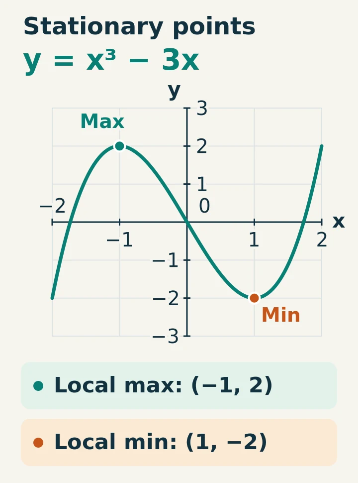
For f(x) = x³ − 3x, differentiate: f′(x) = 3x² − 3 = 3(x − 1)(x + 1). Thus f′(x) = 0 at x = −1 and x = 1.
Evaluate the original function: f(−1) = 2 and f(1) = −2. The second derivative is f″(x) = 6x. It is negative at −1 and positive at 1.
(−1, 2) is a local maximum;
(1, −2) is a local minimum.
The derivative gives a slope, not a point’s height. If the second derivative were zero, this test alone would be inconclusive; examine a derivative sign change or use another valid argument.
3. Separate a definite integral from total area
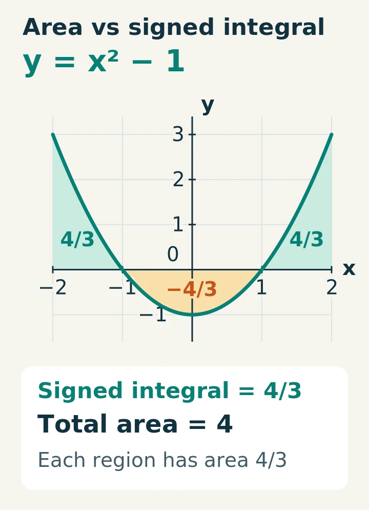
For y = x² − 1 on −2 ≤ x ≤ 2, the graph crosses the x-axis at x = −1 and x = 1. An antiderivative is F(x) = x³/3 − x.
Signed integral = F(2) − F(−2)
= 2/3 − (−2/3) = 4/3.
To find the total area between the curve and the axis, split at both roots. The signed contributions over [−2, −1], [−1, 1] and [1, 2] are 4/3, −4/3 and 4/3.
Total area = |4/3| + |−4/3| + |4/3| = 4 square coordinate units.
Taking the absolute value of the final signed integral would give 4/3 and miss the cancellation. Take absolute values of the separate signed regions instead.
4. Use vector direction and magnitude correctly
Points A and B have position vectors a = (1, 2, −1) and b = (4, 6, 1). The vector from A to B is destination minus start:
AB = b − a = (3, 4, 2)
|AB| = √(3² + 4² + 2²) = √29.
A unit vector pointing from A towards B is (3, 4, 2)/√29. Dividing each component by the magnitude makes its length 1. Reversing direction gives (−3, −4, −2), which has the same magnitude but is a different vector.
5. A particle reverses direction
A particle moves along a straight line with velocity v(t) = t² − 4t + 3 m/s for 0 ≤ t ≤ 3 seconds. Since v(t) = (t − 1)(t − 3), it moves in the positive direction until t = 1 and in the negative direction from t = 1 to t = 3. It is instantaneously at rest at both roots.
An antiderivative of velocity is F(t) = t³/3 − 2t² + 3t. The displacement is F(3) − F(0) = 0. But F(1) = 4/3, so:
Distance = |F(1) − F(0)| + |F(3) − F(1)|
= 4/3 + 4/3 = 8/3 m.
The acceleration is a(t) = 2t − 4 m/s², so it is not constant. Constant-acceleration equations cannot be applied to the whole interval. Zero displacement means the particle returned to its start; it does not mean it never moved.
6. Make a one-sided binomial test and state its conclusion
A process has claimed success probability 0.5. Ten independent trials are observed, with a constant success probability, and nine succeed. Test for an increase at the 5% significance level: H₀: p = 0.5, H₁: p > 0.5.
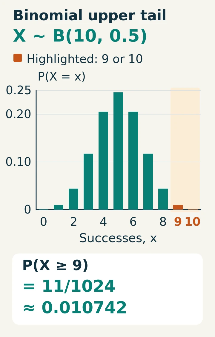
Under H₀, X follows B(10, 0.5). “At least as extreme” in this upper-tail test means nine or ten successes:
P(X ≥ 9) = [C(10, 9) + C(10, 10)] × 0.5¹⁰
= 11/1024 ≈ 0.010742.
Since 0.010742 < 0.05, reject H₀. There is sufficient evidence at the 5% level that the success probability exceeds 0.5, subject to the model assumptions. This does not prove the alternative, and the tail probability is not the probability that H₀ is true.
Eight diagnostic questions with explained answers
Attempt these before opening the answers. Exact forms are preferred where requested; numerical approximations are labelled.
1. Solve (x + 3)/(x − 2) < 0.
The critical values are −3 and 2. The quotient is negative only between them, so −3 < x < 2. Exclude −3 because the inequality is strict, and 2 because the expression is undefined.
2. For y = x³ − 6x² + 9x, find and classify both stationary points.
y′ = 3(x − 1)(x − 3), so x = 1 or 3. The corresponding points are (1, 4) and (3, 0). Since y″ = 6x − 12 is negative at 1 and positive at 3, these are a local maximum and a local minimum, respectively.
3. Find the signed integral and total area of y = x − 1 from x = 0 to x = 3.
An antiderivative is x²/2 − x. The signed integral is 9/2 − 3 = 3/2. Split at x = 1: the area below the axis is 1/2 and above it is 2. Total area = 5/2 square coordinate units.
4. A = (−1, 2, 3) and B = (2, −2, 3). Find AB and a unit vector from A to B.
Subtract coordinates: AB = (3, −4, 0), with magnitude 5. A unit vector in that direction is (3/5, −4/5, 0). Its squared magnitude is 9/25 + 16/25 = 1.
5. A particle has v(t) = 2t − 4 m/s for 0 ≤ t ≤ 5 s. Find displacement and distance.
It turns at t = 2. An antiderivative is t² − 4t. Displacement = 25 − 20 = 5 m. The signed changes are −4 m on [0, 2] and 9 m on [2, 5], so distance = 13 m.
6. A 3 kg particle has forces 14 N east and 5 N west. Find its acceleration.
Take east as positive. Resultant force = 14 − 5 = 9 N. Newton’s second law gives a = 9/3 = 3 m/s² east. Use the resultant force, not the sum of the force magnitudes.
7. For X following B(8, 0.5), calculate P(X ≥ 7). Would seven successes reject p = 0.5 against p > 0.5 at 5%?
The tail is [C(8, 7) + C(8, 8)]/2⁸ = 9/256 = 0.03515625. This is below 0.05, so reject H₀ under the stated binomial assumptions. There is sufficient evidence of an increase; do not say that the increase is proved.
8. X is normally distributed with mean 50 and standard deviation 8. Find P(X > 62).
Standardise: z = (62 − 50)/8 = 1.5. Therefore P(X > 62) = 1 − Φ(1.5) ≈ 0.0668. Here 8 is the standard deviation; the variance is 64. Check which input your calculator asks for.
A final check before you mark
- Domains: exclude zero denominators, check logarithm arguments and give every solution in the requested interval.
- Precision: retain exact fractions or unrounded calculator values during a calculation, then follow the question’s final rounding instruction.
- Units and signs: acceleration has units m/s², displacement is signed, and distance is non-negative.
- Statistics language: define the parameter, choose a justified model, use the correct tail and conclude in context. Failing to reject a null hypothesis is not proof that it is true.
- Grades: a raw percentage is feedback on this attempt, not a universal A-level grade boundary. Use the board’s boundaries for the relevant qualification and series when needed.
Sources & References
AQA owns the official papers and mark schemes below; they remain hosted by AQA. HeLovesMath is an independent educational resource and does not claim endorsement. External resources open in a new tab. Guidance and links checked 5 October 2026; availability and specifications can change.
Original paper archive: match each question paper with its scheme
Five historical series each contain three question papers and three mark schemes. The specimen section adds three sample question papers, three schemes and a commentary. Sample papers illustrate an assessment format; they are not a dated live examination.
June 2022
November 2021
November 2020
June 2019
June 2018
Specimen papers and mark schemes
AQA specimen-paper commentary (PDF)
Official specifications and further study
- AQA 7357 assessment resources: additional papers and examiner reports
- AQA 7357: paper structure, content and weighting
- AQA 7357: scheme of assessment
- AQA: large data set and the 2020 change
- AQA AS Mathematics 7356: separate qualification
- OxfordAQA International Mathematics 9660: separate qualification
- OpenStax Calculus: definite integrals and total area
The worked examples, practice questions and diagrams on this page are original teaching material. Use AQA’s current resources for additional series, examiner reports, the required formulae booklet and the data set for your course.