SAT Math Notes: Complete Guide & Key Topics
This is a comprehensive guide of the math you need to know for the SAT Math Section. It includes step-by-step examples for how to solve for all of the key topics and question types you will encounter.
Keep an eye out for the USEFUL TIPS since they could give you hints for how to solve problems more quickly, even for some of the questions with basic content.
The SAT math section includes problems from the following four general categories, with more specific topics included in each category, as shown below.
|
|
Heart of Algebra
The Heart of Algebra problems make up 18 of 58 questions, or roughly 32.8% of the entire math section. The main topics include:
- Linear equations and inequalities
- Interpreting linear functions
- Systems of linear equations and inequalities
- Basic function notation
- Absolute value functions
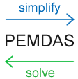
Simplifying Expressions Simplify expressions with the order of operations, PEMDAS.
Simplifying Example: 4(8 – 5) + 9 Subtract 5 from 8. According to the PEMDAS order, first simplify anything inside of the Parenthesis. 4(3) + 9 Multiply 4 by 3. According to PEMDAS, there is nothing left to simplify in the Parenthesis and no Exponents to deal with, so the next step would be to Multiply or Divide. 12 + 9 Add 12 and 9. This is the only step left. 21 | Solving for a Variable Solve for a variable using the reverse order of PEMDAS: SADMEP.
Solving Example: Multiply by 2. There is nothing that can be Added or Subtracted, but there is something that can be Divided or Multiplied, so do that first in this case. 3x – 12 = 18 Add 12. According to the SADMEP order, there is something that can be Subtracted or Added to both sides next. 3x = 30 Divide by 3. According to SADMEP, there is nothing that can be Subtracted or Added to both sides, so the next step would be to Divide or Multiply. x = 10 |


Forms of Linear Equations for Graphing
Linear equations can be expressed in the forms shown below.
*Note: The word “output” is interchangeable with the word “height.”
Slope-Intercept Form
m = slope or rate
b = y-intercept
x = input value of the function | Slope Formula
m = slope
*This form is often used to find the slope when two points are known. | Standard Form
USEFUL TIP: If y is isolated for the standard form, the equation becomes:
where -A/B is the slope, and C/B is the y-intercept. |


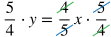
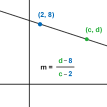
USEFUL TIP: If the coordinates of a point are given but they are in the form of two variables, such as the point (c, d), then you can substitute c as an x value and d as a y value in one of the formulas above to help you solve the problem. Don’t get intimidated if you don’t see numbers as point coordinates, such as (4, 7). You can manipulate other variables in the same way as numbers, even if the answer is written in terms of the variables (see example 4 below).
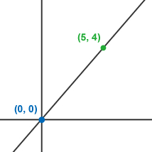
USEFUL TIP: If it’s given that the line goes through the origin, you know that (0, 0) is one of the points on that line, so you can often use that information to get to the answer (see example 3 below).
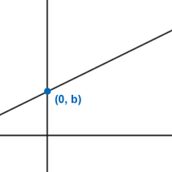
Example 1. The y-intercept is always at (0, b) for y = mx + b. Note that the y-axis is the line x = 0, so the x value will always be 0 for the y-intercept of a graph. By plugging in 0 for x for y = mx + b, you get y = m(x) + b. Therefore, y = b when x = 0. |
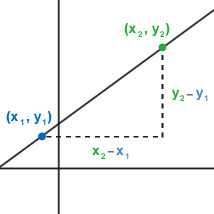
Example 2. Visualization of the “rise” and “run” of a slope, represented by y2 – y1, and x2 – x1, respectively. |
Example 3. When it’s given that the line goes through the origin, you can often use (0, 0) as a point to help solve the problem. |
Example 4. If the coordinates are given as variables, use them as you would numbers to find the slope or other values of a line. |
Interpreting Linear Equations
On the SAT you may need to interpret the meaning of part of a linear equation or its graph in the context of the situation it represents. For problems where the equation is given, it could be of the form y = mx + b, or it could be written in a different form that still represents a linear equation. Variables other than x and y might be used as well.
Imagine this scenario: Betty is selling popcorn at a school event. She spent $12 on cotton candy ingredients and supplies in total, and she is charging $1.50 per cotton candy that she sells, where p is the profit she earns and c is the number of cotton candies sold.
Below are some ways that p as a function of c may be expressed for this situation.
|
|
|
|
|


Those 5 equations all represent the same function, and there are even more ways to rewrite the function. For interpreting linear functions, you will typically have to figure out whether a given part of the function represents the rate or initial condition of a situation.
For example, if the function is written as:

What is the best interpretation of the number -12 in the equation?
A) Betty loses $12 for every cotton candy that she sells.
B) It cost Betty $12 originally to set up her operation.
C) Betty will need to sell 12 cotton candies to break even.
D) There are 12 cotton candies left for Betty to sell.
Answer: B
Explanation: When Betty has sold 0 cotton candies, c = 0. By plugging in 0 for the variable c in the equation, p = -12. This means that her profit when she started is -12 dollars. In other words, she has spent 12 dollars before selling any cotton candies.
USEFUL TIP: If you’re having trouble interpreting parts of a linear function because of its form, take a few moments to rewrite it in the form y = mx + b (slope-intercept form) so that you can quickly tell what the parts of the equation represent.

Finding the Rate:
- It is the value being multiplied by the input variable (the variable on the x-axis) for slope-intercept form.
- For graphs, it is the value of the slope.
- In each of the five equations above, p increases by 1.5, or 3/2, for each increase of 1 for c. Therefore, the rate of change of p in terms of c is 1.5, or 3/2.
Finding the Initial/Starting Condition (Initial Output):
- It is the constant on the side with the input variable for slope-intercept form.
- For graphs, it is the y-intercept.
- In the equations above, p = -12 when c = 0. Therefore, the profit is -12 dollars when 0 cotton candies are sold.
USEFUL TIP: There may be cases where you are asked to solve for p in terms of c. In other words, you would need to isolated the other variable. In those instances, use the Reverse order of PEMDAS (or SADMEP) that was mentioned earlier to isolate the other variable.
For example, solve for c in terms of p (in other words, get c by itself):


For an alternate form, distribute 2/3 to the terms in the parenthesis on the left side.

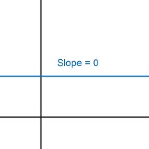
Slopes of horizontal lines are 0. |
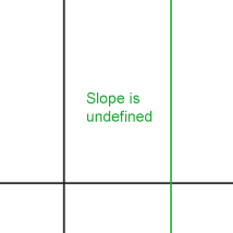
Slopes of vertical lines are undefined. |
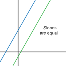
Slopes of parallel lines are equal. |
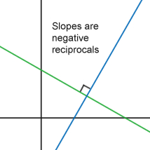
Slopes of perpendicular lines are negative reciprocals. For example: 5/3 and -3/5. |
Systems of Linear Equations
Systems of linear equations are two or more lines that are graphed simultaneously. Solutions for systems of equations are the points where the graphs intersect. There are three possible types of solutions for systems of linear equations.
One solution: The lines intersect at one point.
|
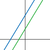
No solutions: The lines intersect nowhere.
|
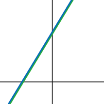
Infinite Solutions: The lines intersect at infinite points (they are overlapping lines).
|

More about Infinite Solutions
- If each of the coefficients and constants of one linear equation are proportional to the corresponding coefficients or constants of another linear equation, the lines will have infinite solutions.
- For example: -2x + 3y = 9 and -4x + 6y = 18 will have infinite solutions because the second equation’s coefficients and constant are all twice the value of the first equation’s.
- Written in y = mx + b form, both equations could be rewritten as y = (2/3)x + 3. In other words, they are the same line.
Graphing Linear Equations
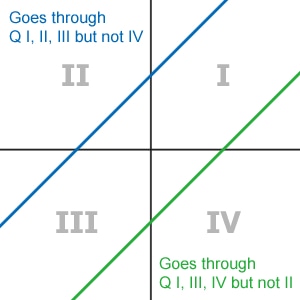
Graphed lines will go through at most only 3 quadrants.
Lines with positive slopes with a positive y-intercept will go through quadrants I, II, and III, but will not go through quadrant IV. Lines with positive slopes with a negative y-intercept will go through quadrants I, III, and IV, but will not go through quadrant II. |
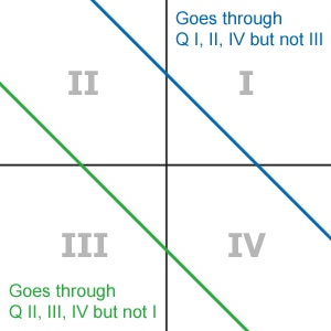
Lines with negative slopes with a positive y-intercept will go through quadrants I, II, and IV, but will not go through quadrant III. Lines with negative slopes with a negative y-intercept will go through quadrants II, III, and IV, but will not go through quadrant I. |
Solving Systems of Equations
As mentioned above, the solution to a system of equations is the point or points where two lines intersect. If you’re given two lines in either the slope-intercept form (y = mx + b) or standard form (Ax + By = C), you can solve for the places the lines intersect by either the Combination Method (sometimes called the Elimination Method) or the Substitution Method.
Combination Method
General process: Make the coefficients of one of the variables opposites, add the equations to cancel out the variable, and solve for the other variable.
Example: | Steps: |
10x + 5y = 40 -6x + 2y = -4 | Multiply either or both equations by a number that makes the coefficients of one of the variables opposite values. In this case, the top equation can be multiplied by 3 and the bottom equation can be multiplied by 5. This will make it so that there is 30x in the top equation and -30x in the bottom equation. |
3•(10x + 5y = 40) 5•(-6x + 2y = -4) | Distribute. |
30x + 15y = 120 -30x + 10y = -20 | Add the left sides together and set them equal to the right sides added together. Notice that 30x and -30x will cancel each other out. |
25y = 100 | Solve for y by dividing both sides by 25. |
y = 4 | Substitute the value of y into one of the original equations. |
10x + 5(4) = 40 | Solve for x. |
10x = 20
x = 2
Since x = 2 and y = 4, the solution to the system of equations is the point (2, 4).
USEFUL TIP: Almost all systems of equations problems can be solved fairly efficiently with the combination method on the SAT.
USEFUL TIP: Using the combination method, if you need to solve for just one variable, multiply the equations by constants that cancel out the other variable.
Substitution Method
General process: Solve for one variable in terms of the other and substitute the value into the second equation.
Example: | Steps: |
3x + y = -10 -4y = -8x – 20 | Solve for y in terms of x in the top equation by subtracting 3x from both sides. |
y = -3x – 10 | Substitute -3x – 10 for y into the bottom equation. |
-4(-3x – 10) = -8x – 20 | Solve for x since it is the only variable in the equation. |
12x + 40 = -8x – 20
20x + 40 = -20
20x = -60
x = -3 | Substitute -3 for x in the other equation (3x + y = -10) to solve for y. |
3(-3) + y = -10
-9 + y = -10
y = -1
Since x = -3 and y = -1, the solution to the system of equations is (-3, -1).
USEFUL TIP: In the problem above, -3 could be substituted into the equation y = -3x -10 to solve for y more quickly.
USEFUL TIP: Sometimes you only need to solve for one variable. Using the substitution method, if you need to just solve for x, first solve for y in terms of x for the first step. If you need to just solve for y, first solve for x in terms of y for the first step.
Function Notation Basics
Function notation is a slightly different method of writing equations than we’ve discussed so far. In basic function notation f(x) (read “f of x”) represents the output of a function. The x inside the parenthesis represents the input of the function. In the regular x and y coordinate graphing system, f(x) takes the place of y, the graph’s output (a.k.a. height).
For example, f(x) = 2x – 5 is the function notation equivalent of y = 2x – 5. And y = -3x + 8 could be written as f(x) = -3x + 8 in function notation.
Although f(x) = “expression” is the basic form of function notation, other letters besides f and x can also be used, just as linear equations can be written with variables other than x and y. For example, y = 4x + 3 could be rewritten as h = 4s + 3, where both y and h refer to the output, and x and s refer to the input of a linear function. Similarly, f(x) = 4x + 3 and g(x) = 4x + 3 and p(a) = 4a + 3 all refer to a function where the input is multiplied by 4 and then 3 is added to the value.
Function notation can also specify certain input and output pairs. Let’s use the function f(x) = 5x + 8 as an example. This function states that the input is multiplied by 5 and then 8 is added to the value. We could say that f(2) = 18. This means that by inputting 2 into the function, the output is 18. We can check this: f(2) = 5(2) + 8 = 18.
Using this same function, f(3) would mean that 3 is the input value. Therefore, f(3) = 5(3) + 8 = 23.
More on Function Notation is given in the Passport to Advanced Mathematics section.
Linear Inequalities in One Variable
Graphing Linear Inequalities in One Variable
When graphing linear inequalities, the collection of all points that make the inequality true are plotted on a number line. For “greater than” or “less than” inequalities, there will be an open (not filled in) point. On the other hand, for “greater than or equal to” or “less than or equal to” inequalities, the corresponding point is closed (filled in).
There is an open (not filled in) circle at x = 3. This might be a representation of the sentence: ”He has more than three dollars.” |
There is a closed (filled in) circle at x = 3. This might be a representation of the sentence: “He has at least three dollars.” |


Notice the difference between these two graphs: the “greater than” graph is not filled at the point x = 3 since plugging in 3 for x would not make the inequality true. 3 is not greater than 3. However, for the “greater than or equal to” graph, plugging in 3 for x would still make the inequality true since 3 is greater than OR EQUAL TO 3.
For graphs that are “less than” or “less than or equal to,” the graph would be filled in on points to the left of a specific value instead of to the right as shown above.
Solving for Linear Inequalities in One Variable
When solving for an inequality, use the same process as solving for a variable in an equation until the variable is isolated. The one major difference is that when multiplying or diving by a negative value, you need to reverse the direction of the inequality sign.
Example 1: 2x + 5 > 17 Subtract 5. 2x > 12 Divide by 2. x > 6 | Example 2: -4x – 2 ≤ 6 Add 2. –4x ≤ 8 Divide by -4 and reverse the inequality sign. x ≥ -2 |
Linear Inequalities in Two Variables
The solution to linear inequalities graphed on an xy-plane is the shaded region of points that make the inequality true. You should be careful to note whether the region to shade should be above or below a certain line and whether the line itself should be a solid line or a dotted line.
Choosing which Region to Shade
- If the inequality starts as y > … or y ≥ … then the region above the line is shaded (for “greater than” or “greater than or equal to”).
- If the inequality starts as y < … or y ≤ … then the region below the line is shaded (for “less than” or “less than or equal to”).
Choosing the Type of Line
- If the inequality starts as y > … or y < … then the line is dotted, since the values for x and y on the line itself do not make the inequality true (for “greater than” or “less than”).
- If the inequality starts as y ≥ … or y ≤ … then the line is solid, since the values for x and y on the line itself make the inequality true (for “greater than or equal to” or “less than or equal to”).
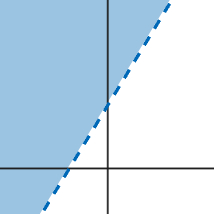
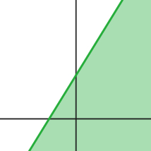
y > 2x + 3 The line is dotted since points on the line do not make the inequality true. The region above the line is shaded since y (the height) is greater than the line. |
y ≥ 2x + 3 The line is filled in since points on the line make the inequality true. The region above the line is shaded since y (the height) is greater than or equal to the line. |
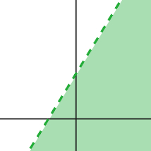
y < 2x + 3 The line is dotted since points on the line do not make the inequality true. The region below the line is shaded since y (the height) is less than the line. |
y ≤ 2x + 3 The line is filled in since points on the line make the inequality true. The region below the line is shaded since y (the height) is less than or equal to the line. |

Systems of Linear Inequalities
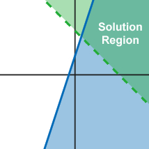
The solution to a system of linear inequalities is the region of points where both inequalities are true at the same time. Two inequalities are graphed together below that illustrates this idea. The inequalities are y ≤ 3x + 1 and y > -x + 2.
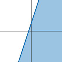
y ≤ 3x + 1 |
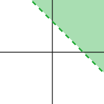
y > -x + 2 |
y ≤ 3x + 1 and y > -x + 2 graphed together. The solution is the overlapping region. |
Absolute Value
Absolute value refers to the magnitude of a value, regardless of its sign. In other words, it is the distance of a value from 0, no matter which direction it is. The symbol for absolute value is two vertical lines. The absolute of x is written as |x|.
For example, the absolute value of -3 is 3 because -3 is 3 units away from 0. This could be written using math symbols as |-3| = 3. On the other hand, 3 is also 3 units away from 0. So |3| = 3 is also true. |-3| = 3 and |3| = 3.
In the equation |x + 6| = 2, there are two possible solutions for x. Think about it this way: if the expression inside the absolute value sign is equal to either 2 or -2, the equation is true. So to solve for x, we can set up two different equations: x + 6 = 2 or x + 6 = -2.
By solving for the two equations, we get x = -4 or x = -8.
Distance-Rate-Time and Work-Rate-Time Problems
The relationship between distance, rate, and time is essentially the same as the relationship between work, rate, and time.
Distance – Rate – Time
Making sense of the equation: If you were to run at 10 miles an hour for 2 hours, you would run 10 miles per hour times 2 hours, or 20 miles total.
If you are given two parts of a D-R-T problem, rewrite d = rt to solve for the remaining variable.
| Work – Rate – Time
Similarly to the D-R-T example, if you were to paint 10 walls an hour for 2 hours, you would paint 10 walls per hour times 2 hours, or 20 walls total.
If you are given two parts of a W-R-T problem, rewrite w = rt to solve for the remaining variable.
|


Problem Solving and Data Analysis
The Problem Solving and Data Analysis problems are only on the Calculator Section of the SAT. The make up 17 of 58 questions, or roughly 29.3% of the entire math section. The main topics include:
- Ratios, rates, and proportions
- Percentages
- Units
- Linear and exponential growth
- Reading table data and graphs
- Data collection, inference, and conclusions
Ratios
A ratio is a comparison of one value to another. It can be written as a fraction, such as 3/4, or with a colon, such as 3:4. Ratios are typically used to compare parts to parts, or parts to wholes.
For example, if you need to make a fruit smoothie that uses 2 strawberries, 5 raspberries, and 6 blueberries, the ratio of strawberries to raspberries would be 2:5 (part to part). The ratio of strawberries to fruit would be 2:13 (part to whole).
USEFUL TIP: If a ratio is given not in its fraction form, turn it into the fraction form first since it will often be easier to use that form to solve a problem.
Rates
Rates are ratios that compare ratios involving two different units of measurement. They often involve time as a unit. When dealing with anything that says, “per minute,” “per week,” per year,” etc., that is a rate.
Rates involving units of time:
| Rates involving units other than time:
|
As you can see in the examples above, the denominator of a rate might not always be a unit of 1.
USEFUL TIP: When asked to find a rate, make sure to carefully check the units and cancel common factors. For example, if revenue increases by $45,000 over 3 years, both the numerator and denominator have a factor of 3 that can cancel. The simplified rate would be $45,000 / 3 years = $15,000 / 1 year.
Unit Rates
Unit rates are rates in which the denominator is written in terms of a unit of 1. For example, 55 miles per hour is a unit rate because it means that an object moves at a rate of 55 miles in one hour.

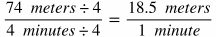
To convert a rate into a unit rate, divide both the numerator and denominator by the value in the denominator.
Example:
A hot air balloon rises 74 meters in 4 minutes. What is the unit rate for its speed of ascent?

Density as a Unit Rate
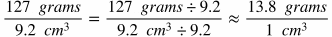
Density is defined as the mass of an object divided by its volume and is typically given as a unit rate.
Example:
If the density of liquid mercury is 13.56 grams per cubic centimeter, would an object that has a mass of 127 grams and takes up 9.2 cubic centimeters float or sink in the mercury?
In order to solve this, you need to determine whether the object’s density is greater or less than that of the liquid mercury’s.
Proportions
Proportions are two or more ratios that are equal. Ratios are proportional if they are equal. Here are examples of proportions:
|
|
|
|


Notice that there can be more than two equal ratios in a proportion, and variables can also be used.
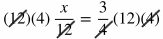
Proportions can often be solved by “cross multiplying.” To cross multiply means to multiply the numerator of one fraction by the denominator of the other fraction and set that equal to the denominator of the first fraction being multiplied by the numerator of the second fraction. This works because if you multiply both sides of the original equation by both denominators, the denominators will cancel out as shown below:
Multiply both sides by both denominators. |
Cancel out the same factors in the numerator and denominator on each side. |
(Previous step shown) |
This shows the original equation when it is cross multiplied. Next, multiply 3 by 12. |
Divide by 4. |
|


In the example above, if you were to start by cross multiplying, you would multiply x times 4 and set that equal to 3 times 12: 4x = 3•12.
This is a good method to use on the SAT to save time.
USEFUL TIP: Solve for proportions by cross multiplying. (Just make sure you understand why it works!)
Another way to deal with a proportion when the unknown value is in the numerator is to multiply both sides by the denominator of the side with the unknown value. The next problem shows this method.
Example:
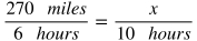
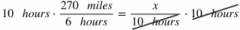
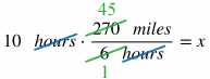
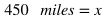
If a man drives 270 miles in 6 hours, at the same rate, how far will he drive in 10 hours?
Remember that proportions are equal ratios, or equal rates. In this scenario, we are dealing with rates. One rate is 270 miles / 6 hours. In the other rate, we aren’t given the number of miles, but we are given the number of hours, so we can use a variable to represent the unknown number of miles and divide it by 10 hours, which becomes x / 10 hours. Then we can set these rates equal to each other to solve for the unknown value:

The key to unit conversions is to make sure that equivalent values are substituted accurately and that units cancel properly during the conversion process.
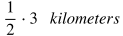
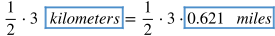
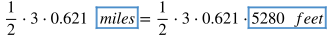
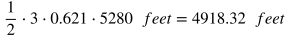
Example problem: If a person runs half of a 3 kilometer race, how many feet would that person have run during that portion of the race?
(1 kilometer = 0.621 miles, and 1 mile = 5280 feet)
To solve this problem, first you can write the original information given and then substitute equivalent values for units until you convert the unit into feet.
For anything other than very common knowledge, problems involving unit conversions will give you information on how one unit converts to another.
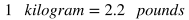
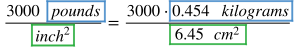
If you need to convert units in the numerator and denominator, the same principle as above applies. In a slightly more complicated example, let’s say that a certain type of glass can support 3,000 pounds per square inch, and you need to find how many kilograms per square centimeter that would be. (1 kilogram = 2.2 pounds, and 1 square inch = 6.45 square centimeters).
In this situation we are given that 1 kilogram = 2.2 pounds. However, since we are given pounds per square inch but we need kilograms per square centimeter, we need to convert pounds into kilograms to start.

Next, substitute 0.454 kilograms for “pounds” and 6.45 cm^2 for “inches^2.”

A percentage is a ratio that means “per 100” or “out of 100.” For example, 32 percent (32%) means 32 out of 100.
It’s often useful to use the decimal version of a percentage when calculating. To turn a percentage into a decimal, divide the percentage number by 100. For example, 57% = 57/100 = 0.57.
To convert between percentages and fractions, use the formula:

Formula | Example Situation | Calculation |
| What is 42% of $280? |
|


| What percent of 60 is 24? |
|


| If a computer’s old version cost $800 when it came out, but the new version costs $920, what percent increase is the new version’s price compared to the old version? |
(This means the price increased by 15%). |

| If a jacket is on sale for 20% off and originally cost $85, what is the new price? |
(Note: The percentage change is -20%, since it is 20% less than the original price.) |


Graphs of Scatterplots
Scatterplots are graphs that typically include these characteristics:
- Data points are plotted on an xy-grid.
- The x and y values represent different units.
- They are often used to find trends or patterns in data with two variables.
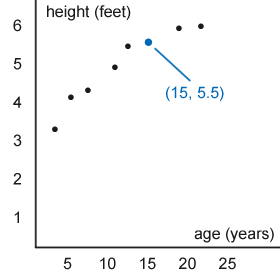
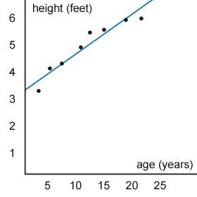
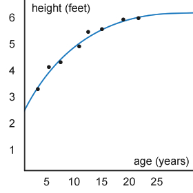
Best-fit Line and Best-fit Curve
An equation that most closely describes the points on a scatterplot is called a best-fit line (for linear models) and a best-fit curve (for non-linear models).
Here is some information you should know about best-fit lines or curves:
- They often do not go through all of the points.
- They do not need to go through any of the points.
- They can be used to estimate where a certain point may be, even though there may not be a point there.
Best-fit Line
| Best-fit Curve
|
Modeling Data
The relationship between two variables can be expressed as an equation that allows you to make a prediction or draw conclusions about the data. Here are three types of models that you are most likely to come across.
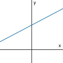
Linear In a linear model, the values increase when the slope is positive. The values decrease when the slope is negative.
m: slope or rate of change b: initial amount (the y-intercept) |
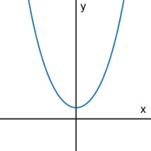
Quadratic In a quadratic model, the shape looks roughly like a “U” and the values change from decreasing to increasing or vice versa. When the coefficient of the x^2 value is positive, the graph opens up and will have a minimum point, as shown above. When the coefficient of the x^2 value is negative, the graph open down and will have a maximum point. The maximum or minimum point of a parabola is called the vertex.
a: if positive the graph opens up, and if negative the graph opens down |
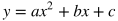
Exponential An exponential function will be a curve where one side “flattens out” while the other side either shoots up or down more and more quickly. Unlike the quadratic model, the values for an exponential function do not change direction and there is no vertex.
a: the initial amount (output value when x = 0) b: common ratio (determines the ratio of one output value to the previous value each time x is increased by 1) |


Association
The association of a model to data describes how closely the data fits the model. If the data fits the model closely, it is called a strong association. If it fits somewhat, it is called a weak association. There is no association if the data does not fit the model at all. Additionally, for linear models, if the model has a positive slope, the association is also called positive. If the model has a negative slope, the association is also called negative.
Below are five associations for linear models.
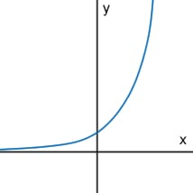
Strong positive association |
Weaker positive association |
No association |
Weaker negative association |
Strong negative association |
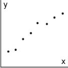
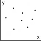
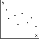
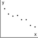
Table data presented as two-way tables allow you to calculate the relative frequency or the conditional probability of an event. The relative frequency is the percentage a sub-group is of the larger group. And a conditional probability is the probability of an event occurring given that some other aspect is already known to be true.
Let’s use this hypothetical situation and the table below to calculate such values: 127 people in a town answered a survey about their age and whether or not they had travelled abroad. The answers are reported in this two-way table.
The rows on the left shows the travel status, while the two middle columns show the age. The totals of each column and row are shown in the margins. | 18 = the number of people younger than 20 who have travelled abroad. 44 = the number of people younger than 20 who have not travelled abroad. 62 = the total number of people under 20. |
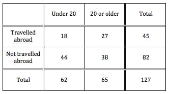
Approximately what percent of the respondents have never travelled abroad? Solution: 82 / 127 is approximately .6456 or 65%. | If a person is chosen at random from those who have travelled abroad, what is the probability that they are 20 or older? Solution: 27 / 45 = 0.6 or 60%. | Those who have travelled abroad or are under 20 make up what fraction of the total respondents? Solution: Therefore, to calculate the answer, we need to add the number of people who have travelled abroad with those under 20, and then subtract 18 so that we don’t double-count the overlap. Travelled abroad (45) + under 20 (62) – travelled abroad AND under 20 (18) = 45 + 62 – 18 = 89. Finally, we need to divide this number by the total number of people to find the fraction who have travelled abroad or are under 20. 89 / 127 |
Term | Definition | Calculation / How to Find the Value |
Mean (Arithmetic Average) | The sum of values divided by the number of values. |
|
Median | The value in a middle of a set of numbers when they are arranged from least to greatest. If there is an even number of terms, take the mean of the two middle terms. | There are 9 numbers in this set. Therefore, the middle value is the fifth number since there are four numbers both below and above the fifth number. The fifth number in this set is 10. |
Mode | The number that appears the most frequently in a set. | 8 is the mode in this set since it appears three times, which is more than any other number appears. |
Range | The difference between the greatest and least value. To find the range, calculate the maximum minus the minimum. | 18 is the maximum, and 5 is the minimum. The range is 18 – 5 = 13. |
You should also understand what standard deviation, confidence intervals, and measurement error are to answer certain questions, but you will not need to calculate their values.
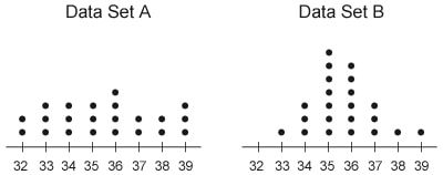
Standard Deviation: A measure of how far data points are spread from the mean of the data. In general, there will be a lower standard deviation if most values are closer to the mean than if they are farther from the mean. For example, this set of data: 8, 8, 9, 10, 12, has a smaller standard deviation than this set: 8, 12, 15, 23, 28. This is because the first set of numbers are all generally closer to the mean than the second set of numbers.
Confidence Intervals: Confidence intervals contain two components: an interval between which a data value is expected to be found and the probability that it will be in that interval. For example, after studying the traffic flow at a certain stop light, it was found that there would be between 410 to 530 cars (the interval) that drive through the light in a day for 95% of days (the probability). Based on this confidence interval, it would be highly likely that on any given day there would be between 410 to 530 cars that drive through the light and a low probability that there would either be less than 410 cars or more than 530 cars that drive through the light.
Measurement Error: The difference between a measured value of quantity and its true measurement. Measurement errors are either:
- Random errors that occur while taking measurements (such as a person accidentally filling out the wrong age).
- Problems with the way data are collected that causes inaccurate results (such as trying to find the average age of people in a town but only asking people at a university, which would not be a representative sample of everyone in the town).
Random errors are often difficult to anticipate and avoid, but care should be taken to collect data in a way that can find accurate or representative answers of the matter being studied.
Data Inferences
Making data inferences means to deduce properties, or make probable guesses, about a population (the entire group) being studied based on the data taken from a sample (a portion of the population). In order to make accurate data inferences, it’s important that the data is taken in a way that would accurately reflect the overall population.
Here are a few general guidelines that should be followed in order to make accurate data inferences.
Sample Size: In general, a sample size of 30 is considered large enough to make fairly accurate calculations for any size population. That said, the larger the sample, the more accurate the statistics are that can be calculated from it.
Randomization: To be a representative sample of a population, the participants of a sample should be chosen using randomizing techniques to avoid bias.
Passport to Advanced Mathematics
The Passport to Advanced Mathematics problems make up 16 of 58 questions, or roughly 27.6% of the entire math section. The main topics include:
- Polynomial factors, graphs, and operations
- Quadratic, exponential, radical, and rational equations and expressions
- Radical and rational exponents
- Structure in expressions and isolating quantities
- Function notation
|
|
|


Each of the polynomials above have x as the variable, but polynomials could have different variables than x as well.
Also, polynomials are typically written with their exponents in descending order. As you can see with the polynomials above, the first term has the greatest power, with each following terms having a lesser power than the one before it. They don’t need to be written in this order, but keeping the way you write polynomials consistent can help in determining key features that they have.
Adding Polynomials To add two or more polynomials, all you need to do is combine like terms.
Rewrite the expression by placing like terms next to each other and in descending order of powers.
Combine like terms.
| Subtracting Polynomials Subtracting polynomials is very similar to adding them. Just make sure to be careful of distributing a negative sign if necessary.
Distribute the negative sign to the terms in the second polynomial and take everything out of the parenthesis.
Rewrite the expression by placing like terms next to each other and in descending order of powers.
Combine like terms.
|


Multiplying Polynomials
When multiplying polynomials, each term of one polynomial needs to be multiplied by each term of the other polynomial. Then the like terms can be combined.
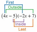
Multiplying Two Binomials For multiplying two binomials (polynomials with two terms) such as for the example below, it can be helpful to remember to multiply the terms in the order FOIL: First, Outside, Inside, Last.
Multiply the terms using the FOIL method.
Combine like terms.
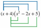
| Multiplying Other Polynomials For multiplying polynomials that are not two binomials, make sure each term of one polynomial is multiplied by each term of the other polynomial. If one polynomial has two terms and the other being multiplied has three terms, there should be a total of 2 x 3 = 6 terms created before combining like terms. This type of example is shown below.
Both x and 4 need to be multiplied by x^2, -2x, and 5.
Rewrite the expression by placing like terms next to each other and in descending order of powers.
Combine like terms.
|


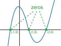
The zeros of a polynomial are the values for x that make the polynomial equal to 0. Other names for the zeros are the x-intercepts, roots, or solutions of the polynomial. The graph of the polynomial shown has three zeros. |
|

This quadratic expression will factor into two binomials. Since the first term is x^2, we can assume that there will be an x in both binomials. At this point we assume the factored form will look something like (x + ?)(x + ?), and we need to find the numbers (called constants) that go in each parenthesis.
Since the constant of the original polynomial is -15, we know that the two constants from the factored form will multiply to -15 when we FOIL. We also know that x is multiplied by each constant, and the original polynomial had a total of 2x. 2x is the value we will get when we combine like terms, which will be our terms with x in them.
This tells us that the two constants will multiply to -15 and add up to 2. To find these numbers, we can think of factors of -15, and see which add up to 2. The only possible pair is -3 and 5. Therefore, the factored form of the quadratic is (x – 3)(x + 5).

To check if this is in fact true, you can use the FOIL method described above to see if the factored form is equivalent to the original quadratic expression.
Finally, to find the zeros of the polynomial, we can use the factored form and set each factor equal to 0 to solve for what values of x make the polynomial equal to 0. Since the zeros (or x-intercepts or roots) are what values of x makes the polynomial equal to 0, we can write 0 = (x – 3)(x + 5).
If either (x – 3) or (x + 5) equals 0, the whole polynomial will equal 0 since the factors are being multiplied by each other. To find the zeros for this quadratic:
- x – 3 = 0, therefore x = 3
- x + 5 = 0, therefore x = -5
The two zeros for x^2 + 2x -15 are x = 3 or x = -5.
Possible Number of Zeros
A polynomial can have at most the same number of zeros as the highest degree of the variable. For example, a quadratic function, which has 2 as the greatest exponent, will have at most 2 zeros. A cubic function, which has 3 as the greatest exponent, will have at most 3 zeros. However, this does not mean that the graph has to have that many zeros.
A function with an odd number as the highest power must have at least 1 zero or as many as up to the highest power. For example, a cubic equation (which has degree 3) could have 1, 2, or 3 zeros.
A function with an even number as the highest power could have no zeros or as many as the up to the highest power. For example, a quartic equation (which has degree 4), could have 0, 1, 2, 3, or 4 zeros.
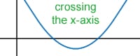
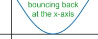
Single zeros (single roots) will “cross” the x-intercept at the zero. For example, for the graph of y = (x – 5)(x – 6), the graph will cross the x-axis at the points x = 5 and x = 6. However, for double zeros (double roots), the graph will not cross the x-axis but will simply “bounce” back from the direction it came. For example, y = (x – 3)(x – 3) has a double root at x = 3. In this case, the graph will come down to touch the x-axis at x = 3 and go back up after that point, but will not cross the x-axis.
In general, single or any odd number of roots at a particular point will cross the x-axis, while double or any even number of roots at a particular point will bounce back from the direction the graph approached the x-axis.
This function has two single roots. They each cross the x-axis. This might be the graph of a function such as y = (x – 1)(x – 3). |
This function has a double root. It bounces back at the x-axis. This might be the graph of a function such as y = (x – 2)(x – 2) = (x – 2)^2. |
There are 3 forms of quadratic equations that you should be familiar with and know how to find the vertex and x-intercepts (a.k.a. zeros, roots, or solutions) for. The vertex is the maximum or minimum of the parabola. The x-intercepts are the values you would input for x to make the height equal to 0. That is, y = 0 or f(x) = 0 at the x-intercepts.
For all of the forms below, when the “a” value is positive, the parabola opens up and it will have a minimum, as shown in the images. When the “a” value is negative, the parabola opens down and it will have a maximum.
|
|

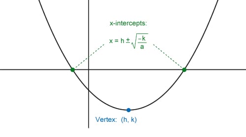
- USEFUL TIP: If you are given the vertex coordinates and one other point of a parabola, you can find the equation of the parabola by solving for the “a” value of the vertex form. In order to do this, substitute the vertex coordinates for h and k, substitute the coordinates of the other point in for x and y, and then the only unknown value left will be “a,” which you can solve for by isolating it in the equation.
For example, if the vertex is (3, -2) and another point on the parabola is (5, 14), then “a” can be solved for by plugging in 3 for h, -2 for k, 5 for x, and 14 for y:
- y = a(x – h)^2 + k becomes 14 = a(5 – 3)^2 – 2
- 14 = a(2)^2 – 2
- 14 = 4a – 2
- 16 = 4a
- 4 = a
Therefore, the equation for the parabola in vertex form is y = 4(x – 3)^2 – 2.
|
|

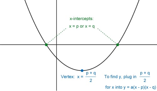
USEFUL TIP: If you are given the x-intercepts and one other point of a parabola, you can find the equation of the parabola by solving for the “a” value of the factored form. In order to do this, substitute in the x-intercepts for p and q, substitute the coordinates of the other point in for x and y, and then the only unknown value left will be “a,” which you can solve for by isolating it in the equation.
For example, if the x-intercepts are at x = -1 and x = 5, and another point on the parabola is (6, 21), then “a” can be solved for by plugging in -1 for q, 5 for p, 6 for x, and 21 for y.
- y = a(x – p)(x – q) becomes 21 = a(6 + 1)(6 – 5)
- 21 = a(7)(1)
- 21 = 7a
- 3 = a
Therefore, the equation for the parabola in factored form is y = 3(x + 1)(x – 5).
USEFUL TIP: Quadratics in standard form may factor and can be rewritten in factored form. If they do, converting the equation to a factored form is often a faster way to solve for the x-intercepts. |
|

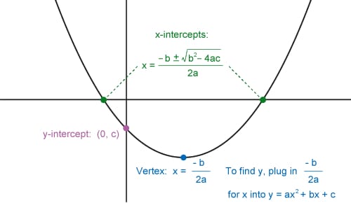
Linear and quadratic systems have solutions where their graphs intersect. To solve for such systems, first make sure both the linear and quadratic equation has isolated one of the variables (typically y), and then set the other expressions equal to each other.
Example: Find the intersections of the following equations.


When x = 2:
| When x = 7:
|
When x = 2, then y = 7. When x = 7, then y = 37. Therefore, the solution to the system are the points (2, 7) and (7, 37). In terms of graphs, this means the line and parabola both go through the points (2, 7) and (7, 37).
For this system, we were able to solve for the quadratic equation that resulted using the standard form and then using the factoring method. However, there are multiple variations to the types of quadratic equations you might be given originally, so make sure to know how to efficiently solve for x using the vertex form, factored form, and standard form as described in the Quadratic Equations section shown above.

In the form above,
- A(t) is the total amount (or output)
- Ao is the initial amount (or amount at time = 0)
- r is the rate of change
- If the rate of change is expressed as a percentage, make sure to convert this to the decimal version of the percentage
- The equation has exponential growth when r > 0 and has exponential decay when r < 0
- t is the time passed (or input variable)
Example problem: If a bank account with $500 earns 8% annual interest and is otherwise left alone, how much money, to the nearest cent, will be in the account after 6 years?
In this example, Ao = $500, r = 0.08 (which is 8%), and t = 6. Plug these values into A(t) = Ao(1 + r)^t to find the solution.

Some situations involving exponential functions are slightly more advanced. These include situations where:
- Case 1: the interest is compounded more than once per time interval t
- Case 2: the initial amount changes by a certain percentage during a time interval either more or less than what is represented by t
For case 1 situations, use the following formula:
In the form above,
Example problem: If an account with $1,600 earns 5% interest compounded quarterly, how much interest, to the nearest cent, will the account earn in 18 years? Notice that this problem is asking how much is earned by only interest, not how much total money is in the account. Since the money is compounded quarterly and t is being measured in units of years, that means that n would be 4 (the money is compounded 4 times per year = compounded n times per t). Ao = 1600
$30,267.23 is the total amount in the account after 18 years. Since we needed to find the amount earned solely by interest, we have to subtract the original $1,600 from the amount in the account to find the answer. $30,267.23 – $1,600 = 28,667.23 | For case 2 situations, use the following formula:
In the form above,
Example problem: If a town’s population is 24,000 people now and is growing by 15% every 10 years, what will the population estimate be, to the nearest person, in 32 years? Since the population is growing in this scenario, b is greater than 1. In fact, it would be 1 + .15 = 1.15. Since b grows 15% every 10 years, c = 10. By using the formula above, we can say that: Ao = 24,000
Rounding to the nearest person would give an estimate of 37,536 people. |


Rule | Example | Explanation |
|
| When multiplying expressions with the same base, add the exponents. |


|
| When dividing expressions with the same base, subtract the exponent of the denominator from the exponent of the numerator. |


|
| When raising an expression with an exponent to a power, multiply the exponents. |


|
| When raising a product to a power, raise each factor to the exponent. |


|
| When raising an expression to a negative exponent, it becomes the reciprocal of the expression with its opposite power. |


|
| An expression to the power of 0 is equal to 1 if the expression itself is not equal to 0. |

Rule | Example | Explanation |
|
| Factors under the radical can be separated into separate radical expressions that are multiplied. |


|
| A quotient under a radical sign can be separated into a quotient of two radical expressions. |


|
| Radical expressions can be combined as like terms if the expressions under the radicals are equal. |


|
| Rational exponents can be turned into radical expressions. The numerator from the exponent is what the radical is raised to. The denominator from the exponent becomes the root of the radical. |


Take the square root of both sides to turn the left side into x. Include the plus or minus sign on the other side during this step.


If you need to simplify an expression with a radical in the denominator (that doesn’t itself simplify), multiply the numerator and denominator by the radical in the denominator. This will allow you to rationalize the denominator. In other words, it will allow you to make the denominator a rational number.
Example problem:


is undefined for where 5x – 10 is less than 0. Set up an inequality to find the undefined values:
5x – 10 < 0
Add 10 to both sides.
5x < 10
Divide both sides by 5.
x < 2
*Note: Negative values under a square root sign can be expressed in terms of i. See the Additional Topics in Math section about Complex Numbers for more about this.
|
|
|


Undefined Values: Rational equations are undefined for values of x (or the input) that make the denominator equal to 0.
For example, the equation

is undefined at the value for x that makes the denominator equal to 0. To find what that value is, set 3x – 2 = 0, and solve for x.
3x – 2 = 0
Add 2 to both sides.
3x = 2
Divide both sides by 3.
x = 2/3
Since plugging in 2/3 for x makes the denominator of the rational equation 0, the expression is undefined at x = 2/3.
USEFUL TIP: When solving for rational equations with multiple terms, you can get rid of all the denominators by multiplying both sides of the equation by the least common multiple of all the denominators.
Example:


Operations with Rational Expressions
Rational expressions can be added, subtracted, multiplied, or divided. Techniques for dealing with each operation involving rational expressions are shown below.
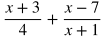
Adding Rational Expressions To add rational expressions, first make a common denominator and then add the numerators.
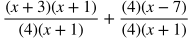
Make a common denominator. In this case it will be (4)(x+1). Multiply the numerators and denominators of both terms by the missing factors of the common denominator.
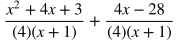
Distribute in the numerators .
Add the numerators and combine like terms.
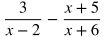
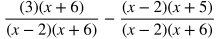
| Subtracting Rational Expressions To subtract rational expressions, first make a common denominator and then find the difference of the numerators.
Make a common denominator. In this case it will be (x-2)(x+6). Multiply the numerators and denominators of both terms by the missing factors of the common denominator.
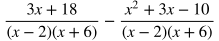
Distribute in the numerators.
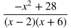
Subtract the second numerator from the first numerator and add like terms. Be careful to make sure to distribute the negative value to each term. When you distribute the negative sign, you will get -x^2, -3x, and +10 for the numerator of the term on the right.
|

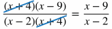
Rational expression factored in the numerator and denominator:
It is easy to tell that the factor (x + 4) cancels out in the numerator and denominator. | The same rational expression not factored:
Unless the numerator and denominator are factored, it is hard to tell how this rational expression will simplify. |

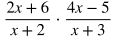
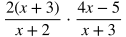
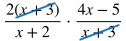
Multiplying Rational Expressions When multiplying rational expressions:
Example:
Put each part in factored form. In this case, 2x + 6 can be factored into 2(x+3).
Cancel out common factors in the numerator and denominator. In this case, x + 3 can be cancelled out.
Multiply across in the numerators and denominators.
Distribute.
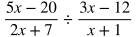
| Dividing Rational Expressions When dividing rational expressions:
Example:
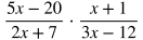
Multiply the first rational expression by the reciprocal of the second.
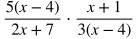
Put each part in factored form.
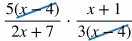
Cancel common factors in the numerators and denominators.
Multiply across in the numerators and denominators.
Distribute.
|


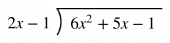
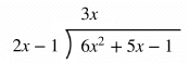
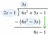
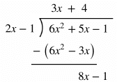
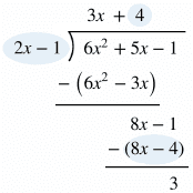
Polynomial Long Division
Rational expressions can be divided using long division in a very similar way to regular long division. Some SAT math problems will require this method to rewrite a rational expression and find an equivalent form.
Example: Use polynomial long division to rewrite the rational expression below.

Function Notation (Extended from Heart of Algebra Section)
Function notation is a method of writing equations for functions. For example, f(x) = 2x – 5 is the function notation equivalent of y = 2x – 5. And y = -3x + 8 could be written as f(x) = -3x + 8 in function notation. Function notation can also be used for quadratics or other types of functions besides linear functions, including piecewise functions (functions with different equations for different domains that are spliced together to make one combined function).
In basic function notation f(x) (read “f of x”) represents the output of a function. The x inside the parenthesis represents the input of the function. In the regular x and y coordinate graphing system, f(x) takes the place of y, the graph’s output, or height.
Although f(x) = [function expression] is the basic form of function notation, other letters besides f and x can also be used, just as linear equations can be written with variables other than x and y. For example, y = 4x + 3 could be rewritten as h = 4s + 3, where both y and h refer to the output, and x and s refer to the input of a linear function. Similarly, f(x) = 4x + 3 and g(x) = 4x + 3 and p(a) = 4a + 3 all refer to a function where the input is multiplied by 4 and then 3 is added to the value.
Function notation can also specify certain input and output pairs. Let’s use the function f(x) = 5x + 8 as an example. This function states that the input is multiplied by 5 and then 8 is added to the value. We could say that f(2) = 18. This means that by inputting 2 into the function, the output is 18. We can check this: f(2) = 5(2) + 8 = 18.
Using this same function, f(3) would mean that 3 is the input value. Therefore, f(3) = 5(3) + 8 = 23.
We could make this even more complicated by evaluating f(a + 4). Since we know the rule of function f is that the input of the function is multiplied by 5 and then 8 is added to it, here is how we can evaluate f(a + 4):
f(a + 4) = 5(a + 4) + 8 = 5a + 20 + 8 = 5a + 28.
Useful Tip: Put a parenthesis around the substituted input value before simplifying to avoid any careless mistakes or distribution errors when dealing with function notation. Using the previous example of f(x) = 5x + 8, when evaluating f(a + 4), the (a + 4) gets substituted for x on the right side of f(x) = 5x + 8. Therefore, substitute exactly (a + 4) with the parenthesis where the x is on the right and then simplify.
There may be more than one place a substitution needs to occur depending on the function. If h(x) = 6x – 12/x, and you were asked to evaluate h(3), you could write: h(3) = 6(3) – 12/(3). This simplifies to 18 – 4 = 14. Notice that when evaluating h(3), (3) was substituted for each place the x was in the original equation on the right side.
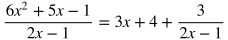
Additional Topics in Math
Additional Topics in Math make up 6 of 58 questions, or roughly 10.3% of the entire math section. The main topics include:
- Geometry: area, volume, triangles, angles, arc lengths, sector areas
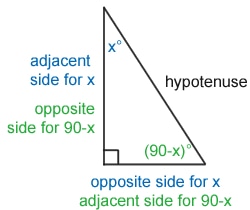
- Right triangle trigonometry
- Circle equations and theorems
- Complex numbers
Knowing the angle relationships below will help you more quickly solve some problems involving diagrams. Many of the explanations involve the word congruent/congruence, so let’s start with an informal definition.
Congruent means that two geometric shapes or objects are the same in size, dimensions, and angle measure (or any combination that may apply). For example, two line segments are congruent if they are the same length. Two angles are congruent if their measures (how many degrees or radians they contain) are the same. Two triangles are congruent if they are the same size and have the same angle measures. Shapes can be congruent even if they don’t face the same direction.
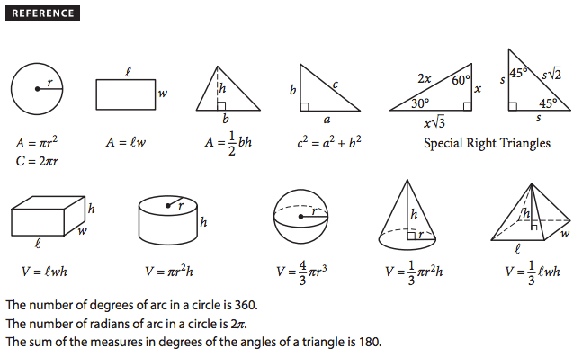
Vertical Angles | Vertical Angles Angles are angles on directly opposite parts of the intersection of two line segments.
|
Corresponding Angles | Corresponding Angles Angles in the same location relative to the intersections formed by the parallel lines and the transversal.
|

Alternate Interior Angles | Alternate Interior Angles Angles on opposite (alternate) sides of the transversal that are on the inside (interior) of the parallel lines.
|

Alternate Exterior Angles | Alternate Exterior Angles Angles on opposite (alternate) sides of the transversal that are on the outside (exterior) of the parallel lines.
|

Same Side Interior Angles | Same Side Interior Angles Angles on the same side of the transversal that are on the inside (interior) of the parallel lines.
|

Same Side Exterior Angles | Same Side Exterior Angles Angles on the same side of the transversal that are on the outside (exterior) of the parallel lines.
|

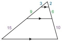
If two lines are intersected by a set of parallel lines, the length of line segments that are created will be proportional. In the case above, each segment on the left is 3/2 times the length of the corresponding segment on the right. |
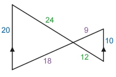
If two triangles (or other polygons) are similar, corresponding angles have the same measures, but the sides are not necessarily the same length. However, the corresponding sides of triangles are proportional in length. In the case above, each side of the triangle on the left is twice the length of its corresponding side on the right. |
Triangle Sum Theorem: The three angle measures of a triangle add up to 180 degrees.
Triangle Inequality Theorem: The sum of the lengths of any two sides of a triangle is larger than the third side.
Side-Angle Relationships: The longest side is opposite the largest angle. The shortest side is opposite the shortest angle.
| Isosceles Triangle Theorems (Isosceles triangles have at least two congruent sides and two congruent angles)
|

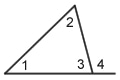
| Exterior Angle Theorem (The exterior angle of a triangle is an angle on the outside of a triangle that makes a linear pair with an angle on the inside of the triangle).
m<1 + m<2 = 180 – m>3. |
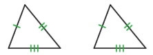
SSS (side-side-side): If all three sides of one triangle are congruent to three corresponding sides of another triangle, the triangles are congruent. |
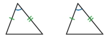
SAS (side-angle-side): If two sides and the included angle of one triangle are congruent to the corresponding parts of another triangle, the triangles are congruent. |
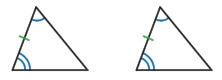
ASA (angle-side-angle): If two angles and the included side are congruent to the corresponding parts of another triangle, the triangles are congruent. |
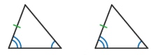
AAS (angle-angle-side): If two angles and a non-included side are congruent to the corresponding parts of another triangle, the triangles are congruent. |
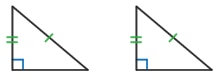
HL (hypotenuse-leg): If the hypotenuse and one leg of a right triangle are congruent to the corresponding parts of another right triangle, the triangles are congruent. | CPCPT: Corresponding parts of congruent triangles are congruent. In other words, if two triangles are shown to be congruent, any other corresponding sides or angles will also be congruent. Information that does NOT Prove Triangle Congruence:
|
|
|
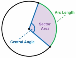
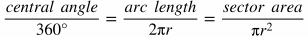
Central Angle: The angle contained between two radii. Arc Length: The length of part of a circle’s circumference. Sector Area: The area of part of a circle (often contained between two radii). The central angle, arc length, and sector area are proportional values. If you know one value, you can find the others using this proportion:
The basic idea behind this proportion is that each fraction contains a part of the circle to the corresponding whole. The fraction of the central angle to the full angle (360°) is the same as the fraction of the arc length to the circumference, which is also the same as the fraction of the sector area to the area of the entire circle. For example, if the central angle is 120°, which is 1/3 of the full angle, then the arc length will be 1/3 of the circumference. USEFUL TIP: The key to solving a problem involving a circle, especially in relation to an arc length or sector area, is often to find the radius. Make sure you know the radius for a problem involving circles if you get stuck. |
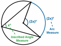
Arc Measure: The angle measure contained within the arc. Inscribed Angle: An angle in the circle with its vertex on the circle. A central angle is equal to the arc measure of the arc it subtends (the arc it creates). However, the arc subtended by an inscribed angle is twice the measure of the inscribed angle. |
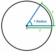
Angles are often measured in units of degrees, but the radian is another unit to measure angles. A radian is the central angle measure that would extend out to fit just between an arc length of exactly one radius length. Whereas degrees divide the circle into 360 equal parts, radians use the radius length placed on the circle as a measuring tool for the central angle. The number of times the radius lengths fits between the angle is the number of radian there are in the central angle. There are 2π radians in a full circle because the radius can fit 2π times around a circle. Remember: C = 2πr. Therefore, 360° = 2π radians. |
|
Converting Between Radians and Degrees
If a radian problem appears on the SAT, it’s highly likely that it will be an angle that is a multiple of 30° or 45°, so it will be good to know what those degrees are in terms of radians.
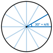
Multiples of 30 Degrees 360° = 2π radians.
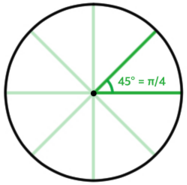
To find how many radians any multiple of 30° is, multiply π/6 by the number of times you would need to multiply 30° by to get that many degrees. For example, 240° is 30° times 8. | Multiples of 45 Degrees 360° = 2π radians.
To find how many radians any multiple of 45° is, multiply π/4 by the number of times you would need to multiply 45° by to get that many degrees. For example, 225° is 45° times 5. |
Radians and Degrees Conversion Proportion
Another way to convert between radians and degree is to use a proportion that relates the two units. By using the ratio of part to whole for the circle, we can set up a proportion to directly convert between radians and degrees.


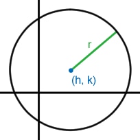
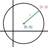
The general equation that describes a circle is
where (h, k) is the circle’s center and r is the length of the radius. A circle with the equation
would have its center at (3, 2) and its radius would be 4. |
|


Completing the Square for Equations of Circles
Completing the square is a technique that can be used to rewrite quadratic equations but it can also be used to manipulate equations for circles to fit the form (x – h)^2 + (y – k)^2 = r^2 if it doesn’t start with that form. The method is called “completing the square” because it takes two terms on one side of an equation (involving a second degree and first degree variable) and rewrites them as a sum or difference being squared.
Steps for Completing the Square (an example is shown below)
- Turn the coefficient of the variable being squared into 1 (if it isn’t already) by dividing both sides of the equation by the value of the original coefficient.
- Move the constant to the other side of the equation from the variables.
- Take half the coefficient of the variable raised to the first power, square the number, and add it to both sides of the equation.
- Factor the side with the variables into a sum squared or a difference squared.
Here is a basic example of completing the square for a quadratic equation without involving the whole equation for a circle:


Now that the equation has completed the square for both the x and y variables, it is in the general equation form for the circle. We can tell that the center is at (5, -4) and the radius is 2.
USEFUL TIP: Don’t mix up the signs for h and k when writing the center. In the example above (x – h) = (x – 5), so h = 5. Also, (y – k) = (y + 4), so k = -4. It’s easy to get the opposite signs by mistake.


For the SAT you should know how to add, subtract, multiply, and divide complex numbers.
To add or subtract complex numbers, the main idea is to simply combine like terms.
Adding Complex Numbers Example:
Rearrange with like terms next to each other (if this step is helpful for you).
Combine like terms.
| Subtracting Complex Numbers Example:
Distribute the negative sign.
Rearrange with like terms next to each other (if this step is helpful for you).
Combine like terms.
|


Multiplying Complex Numbers Example:
FOIL.
Turn i^2 into -1.
Combine like terms.
| Dividing Complex Numbers Example:
Multiply the numerator and denominator by the conjugate of the denominator. The conjugate of the denominator is the expression in the denominator with the sign reversed. The conjugate of 6-2i is 6+2i.
Multiply across in the numerators and denominators by FOILing each.
Notice that the middle terms in the denominators cancel out: 12i – 12i = 0. The purpose of multiplying by the conjugate in the numerator and denominator in the previous step was so that these terms would cancel out and it would eliminate all the imaginary number components in the denominator.
Turn i^2 into -1.
Combine like terms.
Split into two fractions.
Simplify each fraction to make the form a + bi.  |