
Centrifugal Pump Sizing Calculator
Calculate head, pipe loss, pump shaft power, electrical demand, NPSH and curve intersections. Explore seven tools with transparent units, assumptions and worked examples. Use results for learning and preliminary checks; final equipment selection needs verified manufacturer data and professional engineering review.
Calculate Pump Size and Operating Conditions
Select a mode, enter the known values, and calculate pump head, power, NPSH, flow changes, pressure losses, or operating point.
Use SI lengths, density and viscosity. Pressures share one reference. Endpoint velocities are zero at large reservoir surfaces. Use the representative pipe ID for the listed losses; split differing pipe sizes into separate Pipe Loss calculations. Count a fitting in equivalent length or K, never both.
Total Dynamic Head and Pump Power Calculator
Use the Darcy friction factor (four times Fanning). Automatic friction stops in the transitional range 2300 ≤ Re < 4000; manual mode requires a justified factor.
Pipe Friction Loss and Pressure Drop Calculator
This is a large suction-reservoir model with negligible free-surface velocity. Both pressure inputs are absolute. Static suction head is positive above the pump datum and negative for suction lift. The entered ratio is a comparison, not a safety certification.
NPSH Available Calculator
These are corresponding pump-curve points at approximately constant efficiency. The actual operating point requires a new system-curve intersection. Impeller trimming is a limited same-casing approximation.
Pump Affinity Laws Calculator
A simple declining quadratic pump curve and rising quadratic system curve are assumed. Use a nonnegative static head and an actual rated reference flow. Illustrative results cannot replace a manufacturer curve.
Pump Curve and System Curve Operating Point Calculator
This mode finds inside diameter from the target velocity you choose. Length is recorded for context; use Pipe Loss to calculate friction. No universal safe target velocity is assumed.
Inside Diameter from Target Velocity
Use best-efficiency-point (BEP) conditions and head per stage. nq uses total pump flow; suction nss uses flow per eye. These metric indices use rpm, m³/s and metres and are not dimensionless.
Pump Specific Speed and Suction Specific Speed Calculator
Diagram and Calculation Details
What does centrifugal pump sizing actually determine?
A centrifugal pump sizing calculation starts with a required flow rate and estimates the head needed to move that flow through a particular system. It then estimates power and checks suction conditions. A useful preliminary result is a duty statement such as “35 L/s at 63.6 m of head,” accompanied by the fluid properties, operating range and NPSH available.
Head is energy per unit weight of liquid, expressed in metres. It includes elevation, pressure and motion. A pump developing 40 m of head does not necessarily lift liquid vertically by 40 m: some of that energy may maintain vessel pressure or overcome pipe resistance.
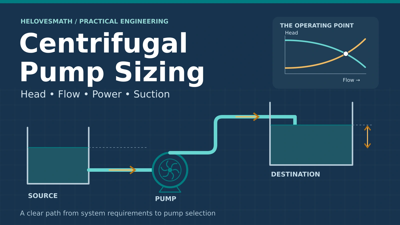
The desired duty point and the actual operating point are different ideas. The desired point comes from the process requirement. The actual point occurs where the pump's head–flow curve crosses the system's head–flow curve. A power estimate alone cannot establish whether a particular pump will deliver the required flow.
This lesson connects the seven calculator modes above. It uses steady, incompressible, single-phase flow and circular pipes as its basic model. The examples are teaching calculations, with stated assumptions, rather than equipment selections.
How to use the centrifugal pump sizing calculator
- Define the endpoints. Mark the source surface or inlet section, the destination surface or outlet section, and one elevation datum. Record what the pressure at each endpoint represents.
- Set the flow and pressure units before entering numbers. Changing a unit converts the existing numerical inputs and clears the old result; calculate again in the current mode. Read each field label again after changing units. Use actual pipe inside diameter, not nominal pipe size.
- Enter properties for the liquid's operating condition. Density, viscosity and vapor pressure can change with temperature and composition. The default water-like values are examples.
- Calculate the separate checks. Flow and TDH, suction conditions, shaft demand and the operating point answer different questions. Completing one does not complete the others.
- Test the range. Repeat for low source level, high destination pressure, maximum temperature, fouled piping and other credible operating cases. Keep each case's inputs with its results.
| Mode | Main question | Important limitation |
|---|---|---|
| Pump Sizing | What head and power does a specified flow require? | One representative pipe diameter; enter the endpoint velocities and calculate additional pipe sections separately. |
| Pipe Loss | How much head is lost in a pipe and its fittings? | Automatic mode rejects Re from 2,300 to below 4,000; any manual Darcy factor needs justification. |
| NPSH | How much suction head remains above vapor pressure? | Uses source-surface absolute pressure and suction-side losses only; margin criteria are application-specific. |
| Affinity Laws | How might corresponding curve points move? | The new system operating point must still be found. |
| System Curve | Where do simplified pump and system curves cross? | Two quadratic curves cannot reproduce every real pump or pipe network. |
| Pipe Diameter | What inside diameter gives a chosen velocity? | The velocity target is an input, not a universal design limit. |
| Specific Speed | What comparative index describes the pump duty? | Use the stated units, best-efficiency-point data and appropriate stage/eye basis. |
Quick conversions: 1 m³/s = 1,000 L/s = 3,600 m³/h; 1 bar = 100 kPa = 100,000 Pa. Enter 72% as 72 in a percentage field, but use 0.72 in a hand calculation. Dynamic viscosity μ is in Pa·s; 1 mPa·s = 0.001 Pa·s. Kinematic viscosity ν is a different quantity: ν = μ/ρ, in m²/s.
Pump sizing formulas and symbols
Use Q in m³/s, diameter D and length L in m, density ρ in kg/m³, dynamic viscosity μ in Pa·s, pressure p in Pa and gravity g in m/s². These examples use g = 9.81 m/s². Efficiencies are fractions in the equations.
H = (p₂ − p₁)/(ρg) + (z₂ − z₁) + (v₂² − v₁²)/(2g) + hL
H is pump total head. The total irreversible loss hL includes pipe-wall losses and local losses between the chosen endpoints. The velocity term shown uses a kinetic-energy correction factor of 1, an approximation commonly used for turbulent-flow calculations.
A = πD²/4; v = Q/A; Re = ρvD/μ
hf = f(L/D)v²/(2g); hm = ΣK · v²/(2g)
hL = hf + hm; Δploss = ρg hL
f is the dimensionless Darcy friction factor; K is a dimensionless local-loss coefficient referenced to a specified pipe velocity. A single ΣK expression assumes the coefficients share that velocity basis.
Phyd = ρgQH
Pshaft = Phyd/ηp; Pelectric = Pshaft/ηm
The answers are in watts. Divide by 1,000 for kW. These expressions omit separate coupling, gearbox or drive losses; include their efficiencies when relevant.
NPSHa = (psurface,abs − pv,abs)/(ρg) + zs − hL,s
zs is source liquid level above the pump's NPSH datum, positive for a flooded suction and negative for a suction lift. hL,s includes all losses from the source surface to the suction measurement section. Source-surface velocity is assumed negligible.
r = N₂/N₁; Q₂ = rQ₁; H₂ = r²H₁; P₂ ≈ r³P₁
Hpump = H₀ − aQ²; Hsystem = Hstatic + KsysQ²
Qop = √[(H₀ − Hstatic)/(a + Ksys)]
The last expression describes positive forward flow when H₀ > Hstatic and a + Ksys > 0. Ksys is a system-curve coefficient with units of s²/m⁵ when Q is in m³/s. It is different from a dimensionless fitting K.
D = √[4Q/(πvtarget)]
nq = N√Q/H3/4; nss = N√(Q/neyes)/NPSH33/4
Here N is in rpm, Q is total pump flow in m³/s, head is per stage in m, NPSH3 is in m, and neyes is 1 for single suction or 2 for symmetric double suction. The calculator calls the first index “metric specific-speed index nq.” Its numerical value depends on this unit convention; it is not a dimensionless index.
Build total dynamic head without losing the pressure reference
Choose endpoints before adding head terms. Between two large reservoirs, the surface velocities are usually negligible. Between two equal-diameter pipe sections carrying the same flow, their velocity heads cancel. A discharge jet or unequal endpoint diameters can leave a significant velocity-head difference.
Enter v₁ and v₂ for the endpoints you chose. Use zero for each large-vessel surface when its velocity is negligible. If the destination is a jet, enter its outlet velocity to account for the remaining kinetic energy. If the destination is a large receiving tank, account for the relevant exit loss instead. Do not charge the same dissipation twice by mixing those two endpoint choices.
Gauge pressure versus absolute pressure
Gauge pressure is relative to local atmospheric pressure; absolute pressure is relative to vacuum. For a common atmospheric reference, pabs = pgauge + patm. The TDH pressure difference may use two absolute pressures or two gauge pressures referenced consistently. Never subtract one absolute pressure from one gauge pressure.
For example, 250,000 Pa absolute minus 101,325 Pa absolute is 148,675 Pa. The equivalent gauge-pressure pair is 148,675 Pa gauge and 0 Pa gauge when atmospheric pressure is 101,325 Pa. Entering 250,000 Pa gauge instead describes a different destination pressure.
Elevation is the vertical difference z₂ − z₁, not the pipe's total length. A horizontal 100 m pipe can have zero elevation rise and substantial friction. In a closed circulation loop returning to the same pressure and elevation, net static terms cancel around the loop, although friction remains.
The quantity ρgH is a pressure equivalent of total pump head. It equals a measured static pressure rise across the pump only when differences in measurement-section elevation and velocity head are accounted for appropriately.

Pipe friction, fittings and Reynolds-number limits
Calculate velocity first because it appears in both Reynolds number and loss equations. For a given Q, doubling D gives four times the area and one quarter of the velocity. With f held constant, substituting v = 4Q/(πD²) into Darcy–Weisbach gives hf proportional to LQ²/D⁵. This strong diameter dependence explains why a small pipe can dominate the head requirement.
Which friction factor belongs in the equation?
- Fully developed laminar flow: f = 64/Re for a circular pipe.
- Turbulent flow: the automatic calculation uses the Swamee–Jain approximation shown below, with roughness ε and diameter D in the same units.
- Transition: roughly Re = 2,000–4,000 is a region in which the flow state and calculated loss are less certain. A smooth numerical answer does not remove that uncertainty.
f ≈ 0.25 / {log₁₀[ε/(3.7D) + 5.74/Re0.9]}²
The calculator rejects automatic friction results for 2,300 ≤ Re < 4,000. Pipe Loss mode allows a manually supplied Darcy factor for a justified sensitivity calculation. Even near the lower transition boundary, the real flow conditions deserve review: an automatic formula choice is not a physical validation of the flow state.
Darcy and Fanning factors differ by four: fDarcy = 4fFanning. A Fanning value entered into this calculator's Darcy field underestimates straight-pipe loss by a factor of four.
Count each loss once
Use either a fitting's K value or its equivalent pipe length for that same fitting. Adding both duplicates the loss. The word “minor” refers to localized losses, not necessarily to a small contribution: a throttled valve can exceed the loss of a long pipe.
For several diameters, calculate each section using its own velocity, length and friction factor, then sum the head losses. Use each fitting coefficient's stated reference velocity. One average diameter or an unqualified combined K is generally insufficient for a branched or changing-diameter network.
Hydraulic power, shaft demand and motor input are different
The liquid receives hydraulic power. The pump shaft supplies more power because ηp is below 1. The motor draws still more electrical power because ηm is below 1. In this lesson, “brake power” and “pump shaft demand” mean the same mechanical input to the pump.
A motor's nameplate kW or horsepower rating ordinarily describes its mechanical output. Compare it with the shaft load, including relevant transmission losses and duty requirements. Electrical input is useful for estimating energy use; it is not the motor's mechanical rating. For constant input power, energy in kWh equals electrical kW multiplied by operating hours.
What does service factor mean?
Motor service factor describes a manufacturer's permitted loading capability under specified conditions. It is not another efficiency and should not automatically multiply normal running energy demand. Temperature, cooling, voltage, drive operation and the manufacturer's instructions affect whether that capability is usable.
The calculator reports a separate planning shaft-power allowance: Pshaft × M, where M is the chosen allowance multiplier. This allowance is separate from the motor's nameplate service factor and from normal electrical demand. It remains a planning value; check maximum shaft demand over the complete intended operating range before selecting a motor.
Changing pump efficiency from 72% to 60% at unchanged hydraulic duty increases shaft demand by 0.72/0.60 = 1.20, or 20%. Using a convenient efficiency everywhere on a curve can therefore hide a meaningful motor-load change.
NPSH available and the limits of a margin check
NPSH available describes suction total head above the liquid's vapor-pressure head. It is calculated from the installation. NPSH required is supplied for the pump at a stated flow, speed and test basis. Always use absolute pressure for the source pressure and vapor pressure in the NPSH calculation.
At a suction measurement section on the pump datum, the same quantity can be expressed as NPSHa = ps,abs/(ρg) + vs²/(2g) − pv,abs/(ρg). This is a different starting point from the source-vessel formula. Do not enter measured suction-flange pressure as source-surface pressure and then subtract upstream suction losses again.
Published NPSH3 identifies a test condition with a 3% head reduction caused by cavitation. It is not the onset of cavitation and does not guarantee cavitation-free operation. Confirm whether a manufacturer's “NPSHr” curve is NPSH3 or includes a different allowance.
Two useful arithmetic checks are the absolute margin NPSHa − NPSHr, in m, and the ratio NPSHa/NPSHr. No single ratio, including 1.10, is a universal acceptance criterion. The required margin depends on the pump, liquid, service and operating region.
Evaluate the minimum source level, lowest source absolute pressure, highest relevant vapor pressure and realistic suction losses. A clogged strainer or lowered tank level can consume margin even when the pump and discharge piping are unchanged. These checks supplement manufacturer and application-specific review.

Affinity laws predict corresponding points; curves predict operation
For the same pump and impeller, a speed ratio r maps a corresponding flow to rQ and its head to r²H. With approximately unchanged efficiency and density, shaft power scales as r³. These relationships help estimate a changed pump curve.
The system still imposes its own head requirement. Re-intersect the changed pump curve with the system curve to find the new operating point. Simple proportional flow reduction is especially misleading when a substantial static head remains as speed falls. Example 5 demonstrates the difference numerically.
Impeller trimming is a separate approximation. The familiar Q ∝ D, H ∝ D² and P ∝ D³ rules can estimate small trims in a given casing, subject to manufacturer limits. Scaling an entire geometrically similar pump is different: the full similarity relations include Q ∝ ND³ and P ∝ N³D⁵ at fixed density. Do not apply one diameter rule to the other problem.
Read the simplified system-curve inputs correctly
In the quadratic model, H₀ is pump shutoff head. A second pump point supplies a = (H₀ − Hrated)/Qrated². A system point supplies Ksys = (Hsystem,rated − Hstatic)/Qrated². Use the same reference flow for both points.
Here Hstatic includes any fixed elevation and fixed pressure-head requirement. A purely quadratic friction term assumes the loss coefficient is approximately constant over the range. Laminar flow, changing valve positions, pressure-dependent demands and network branches can require a different model.
If pump shutoff head is below the system's static requirement, this model has no positive forward-flow intersection. A displayed zero must not be interpreted as a usable duty point. Real operation also requires checking the manufacturer's allowable region, minimum flow and power curve.

Six fully worked centrifugal pump sizing examples
The following values are chosen for calculation practice. Carry unrounded values between steps; the displayed results are rounded. Examples 1 and 2 share a pipeline so the loss calculation can be checked independently.
Example 1: TDH, hydraulic power, shaft power and electrical demand
Given: Q = 0.035 m³/s, ρ = 1,000 kg/m³, z₂ − z₁ = 22 m, p₁ = 101,325 Pa absolute and p₂ = 250,000 Pa absolute. The source and destination are large vessels, so endpoint velocity heads are negligible. Total pipe and local losses from Example 2 are 26.399245 m. Pump efficiency is 72%; motor efficiency is 92%.
- Pressure difference: Δp = 250,000 − 101,325 = 148,675 Pa.
- Pressure head: Δp/(ρg) = 148,675/(1,000 × 9.81) = 15.155454 m.
- Total head: H = 22 + 15.155454 + 26.399245 = 63.554698 m.
- Hydraulic power: Phyd = 1,000 × 9.81 × 0.035 × 63.554698 = 21,821.506 W = 21.822 kW.
- Shaft demand: Pshaft = 21.821506/0.72 = 30.308 kW.
- Motor electrical input: Pelectric = 30.307647/0.92 = 32.943 kW.
Interpretation: the estimated duty is 35 L/s, or 126 m³/h, at 63.555 m head. A planning shaft allowance of M = 1.15 gives 30.307647 × 1.15 = 34.854 kW. This is an allowance on mechanical demand, while normal estimated electrical input remains 32.943 kW. It does not verify a motor rating or its allowable service-factor loading; review the full load envelope.
Calculator check: use the Pump Sizing inputs above together with L = 120 m, D = 0.10 m, μ = 0.001 Pa·s, ε = 0.000045 m and ΣK = 5. Set the flow unit to m³/s and pressure unit to Pa, and enter v₁ = v₂ = 0 for the vessel surfaces.
Example 2: Pipe velocity, friction factor, head loss and pressure loss
Given: Q = 0.035 m³/s, D = 0.10 m, L = 120 m, ρ = 1,000 kg/m³, μ = 0.001 Pa·s, ε = 0.000045 m and ΣK = 5. The K total includes the local losses required by the chosen endpoints; no fitting is also included as equivalent length.
- Area: A = π(0.10)²/4 = 0.007853982 m².
- Velocity: v = 0.035/0.007853982 = 4.456338 m/s.
- Reynolds number: Re = 1,000 × 4.456338 × 0.10/0.001 = 445,634, well above the transitional range.
- Relative roughness: ε/D = 0.000045/0.10 = 0.00045. Swamee–Jain gives f = 0.25/{log₁₀[0.00045/3.7 + 5.74/(445,633.841)0.9]}² = 0.017568.
- Velocity head: v²/(2g) = 4.456338²/19.62 = 1.012179 m.
- Major loss: hf = 0.017567997 × (120/0.10) × 1.012179 = 21.338350 m.
- Local loss: hm = 5 × 1.012179 = 5.060895 m.
- Total: hL = 26.399245 m; Δploss = 1,000 × 9.81 × 26.399245 = 258,977 Pa ≈ 258.977 kPa.
Interpretation: the straight-pipe loss is about four times the local loss here. Changing pipe diameter deserves investigation because velocity is high and the friction contribution exceeds the 22 m elevation rise. This numerical comparison does not establish an acceptable velocity for a particular service.
Example 3: NPSH, suction lift and a changing source level
Given: source pressure = 101,325 Pa absolute, vapor pressure = 3,169 Pa absolute, ρ = 1,000 kg/m³, source level = 2 m above the pump datum, suction losses = 1.2 m and manufacturer NPSHr = 3.0 m at the evaluated duty.
- Pressure head above vapor pressure: (101,325 − 3,169)/9,810 = 10.005708 m.
- Available NPSH: 10.005708 + 2 − 1.2 = 10.805708 m.
- Absolute margin: 10.805708 − 3.0 = 7.805708 m.
- Margin ratio: 10.805708/3.0 = 3.601903.
Now lower the liquid surface to 3 m below the pump datum and increase suction losses to 3 m, keeping the other teaching inputs unchanged. NPSHa = 10.005708 − 3 − 3 = 4.005708 m; the margin becomes 1.005708 m and the ratio 1.335236.
Interpretation: a 5 m level reduction plus 1.8 m extra loss removed 6.8 m of available NPSH. Both cases have positive arithmetic margins, but neither is approved by that fact alone. Confirm the required margin and whether the quoted 3 m curve value is NPSH3.
Example 4: Speed affinity laws at corresponding points
Given: at N₁ = 1,750 rpm, a pump-curve point has Q₁ = 0.035 m³/s, H₁ = 45 m and shaft power P₁ = 21.5 kW. Estimate its corresponding point at N₂ = 1,450 rpm, keeping the same impeller and assuming unchanged density and efficiency.
- Speed ratio: r = 1,450/1,750 = 0.828571429.
- Flow: Q₂ = 0.035r = 0.029 m³/s = 29 L/s.
- Head: H₂ = 45r² = 30.893878 m.
- Shaft power: P₂ = 21.5r³ = 12.230052 kW, a 43.116% reduction at these corresponding points.
Interpretation: these are mapped pump-curve points. The 29 L/s value is not a confirmed delivery rate in an unchanged installation, and the calculated percentage is not a guaranteed site energy saving. The next example performs the missing system-curve check.
Example 5: Find the operating point, then reduce speed
Given: a pump has shutoff head H₀ = 65 m and head 42 m at Qref = 0.040 m³/s. The system requires 22 m at zero flow and 45 m at the same reference flow. Fit the calculator's quadratic models.
- Pump coefficient: a = (65 − 42)/0.040² = 14,375 s²/m⁵.
- System coefficient: Ksys = (45 − 22)/0.040² = 14,375 s²/m⁵.
- Equate the heads: 65 − 14,375Q² = 22 + 14,375Q², so 28,750Q² = 43.
- Operating flow: Q = √(43/28,750) = 0.038673663 m³/s = 38.674 L/s.
- Operating head: H = 22 + 14,375(0.038673663)² = 43.5 m. The pump equation also gives 43.5 m.
- Estimated shaft demand: with ρ = 1,000 kg/m³ and ηp = 0.72, Pshaft = 1,000 × 9.81 × 0.038673663 × 43.5/0.72 = 22.921 kW.
Reduce speed to 80% of its original value. Scale the entire pump curve: Hnew(Q) = 0.8²Hold(Q/0.8) = 41.6 − 14,375Q². Keep the system curve unchanged.
The new intersection satisfies 41.6 − 14,375Q² = 22 + 14,375Q². Therefore Q = √(19.6/28,750) = 0.026110135 m³/s = 26.110 L/s, and H = 31.8 m. With the same illustrative 72% efficiency, shaft demand is 11.313 kW.
Check the tempting shortcut: multiplying the original operating flow by 0.8 gives 30.939 L/s and its mapped pump head is 27.84 m. But the system needs 35.76 m at that flow. Those heads differ by 7.92 m, so that mapped point cannot be the new intersection.
Example 6: Velocity-based pipe diameter and specific speed
Part A, pipe diameter: for Q = 0.035 m³/s and an illustrative target velocity of 2.0 m/s, D = √[4 × 0.035/(π × 2.0)] = 0.149270533 m = 149.271 mm. If an available pipe has an actual inside diameter of 0.150 m, its velocity is 4 × 0.035/[π(0.150)²] = 1.980595 m/s. With ρ = 1,000 kg/m³ and μ = 0.001 Pa·s, Re = 297,089.
This establishes the velocity for a known inside diameter. It does not choose a pipe schedule, pressure class or material, and 2.0 m/s is a practice target rather than a universal recommendation. Recalculate losses and suction conditions using the proposed pipe.
Part B, specific speed: take a single-stage, single-entry pump's best-efficiency-point data as N = 1,750 rpm, Q = 0.035 m³/s and H = 45 m. Then nq = 1,750√0.035/450.75 = 18.843548 in the rpm–m³/s–m convention. With NPSH3 = 3 m and the single-eye setting, nss = 1,750√0.035/30.75 = 143.625360. For a symmetric double-suction impeller, the per-eye flow is 0.035/2 = 0.0175 m³/s; the per-eye suction specific speed would be 143.625360/√2 = 101.558466.
The same hydraulic duty gives a pump specific-speed value of approximately 973.180 when flow is in US gpm and head in ft, about 51.645 times the SI-flow numerical value. The pump has not changed; the convention has. For multistage or double-entry pumps, establish head per stage and the required per-eye flow convention before comparing indices.
Practice: check your pump-sizing reasoning
Use ρ = 1,000 kg/m³ and g = 9.81 m/s² unless a question says otherwise. Try each calculation before opening its answer.
Convert the flow. A transfer system requires 72 m³/h. What are the flow rates in m³/s and L/s?
Show answer and explanation
Q = 72/3,600 = 0.020 m³/s. Multiplying by 1,000 gives 20 L/s. Dividing by 60 would convert hours to minutes, which is not the seconds-based unit used by ρgQH.
Combine head terms. A source is open to atmosphere. The destination is 12 m higher and needs 150 kPa gauge. Total loss is 3 m and endpoint velocities are negligible. Find TDH.
Show answer and explanation
Both pressures can be expressed as gauge values: p₁ = 0 and p₂ = 150,000 Pa. H = 150,000/9,810 + 12 + 3 = 30.291 m. Atmospheric pressure does not need to be added to this consistently referenced pressure difference.
Separate the power quantities. Q = 0.010 m³/s, H = 25 m, pump efficiency = 70% and motor efficiency = 90%. Find hydraulic, shaft and electrical power.
Show answer and explanation
Phyd = 1,000 × 9.81 × 0.010 × 25 = 2.4525 kW. Pshaft = 2.4525/0.70 = 3.5036 kW. Pelectric = 3.503571/0.90 = 3.8929 kW. Efficiencies are divided out as you work upstream toward the energy source.
Find the hidden factor of four. A reference supplies a Fanning friction factor of 0.005. What value belongs in the calculator's manual Darcy field?
Show answer and explanation
Enter 0.020, since fDarcy = 4fFanning. Darcy–Weisbach loss is proportional to f, so entering 0.005 would report only one quarter of the correct straight-pipe loss for the same inputs.
Question a precise output. A pipe calculation gives Re = 3,000. Is either f = 64/Re or a turbulent correlation a dependable exact answer?
Show answer and explanation
No. This is in the transitional range. The laminar expression gives 64/3,000 = 0.02133, but that number does not establish that the real flow is laminar. Investigate the flow conditions and use an appropriate method or sensitivity range; additional displayed decimals do not resolve the uncertainty.
Convert suction pressure correctly. Source pressure is −20 kPa gauge while local atmospheric pressure is 95 kPa absolute. Vapor pressure is 5 kPa absolute, the surface is 1 m above the pump datum, and suction loss is 2 m. Find NPSH available.
Show answer and explanation
Source absolute pressure = 95 − 20 = 75 kPa. NPSHa = (75,000 − 5,000)/9,810 + 1 − 2 = 6.136 m. Using −20 kPa directly would mix a gauge pressure with an absolute vapor pressure.
Check a speed increase. Speed rises by 10% with the same impeller. What are the ideal corresponding-point flow, head and power multipliers?
Show answer and explanation
r = 1.10, so the multipliers are 1.10, 1.21 and 1.331. That means 10% more flow, 21% more head and 33.1% more shaft power at corresponding points under the affinity assumptions. The actual new flow still needs a pump–system intersection.
Test whether the pump can overcome static head. A simplified pump curve is H = 18 − 5,000Q² and the system curve is H = 22 + 8,000Q², with Q in m³/s and H in m. What is the positive operating flow?
Show answer and explanation
There is no positive forward-flow intersection. Equating the curves gives 13,000Q² = −4, which has no real Q. The pump's 18 m shutoff head is already below the 22 m static requirement. Taking a square root after forcing the numerator to zero would hide the failed duty check.
Common centrifugal pump sizing mistakes
- Using vertical rise as the whole TDH: include endpoint pressure requirements, losses and any remaining velocity-head difference.
- Mixing pressure references: keep both TDH pressures on one basis; use absolute pressures for NPSH.
- Confusing nominal pipe size with inside diameter: wall thickness changes area, velocity and loss.
- Counting fittings twice: use equivalent length or K for a particular fitting, not both.
- Trusting transitional-flow precision: Re near 3,000 deserves a method check, not just more decimal places.
- Calling electrical input the motor output rating: separate shaft load, motor input and any stated allowance.
- Treating NPSH3 as cavitation-free: it is a head-drop test criterion; adequate margin requires further assessment.
- Using one efficiency or one operating condition everywhere: review the relevant curves and the full expected range.
- Reading scaled affinity flow as delivered flow: the changed pump curve still has to meet the system curve.
- Comparing bare specific-speed numbers: state units, stage basis, flow-per-eye convention and the point used.
Centrifugal pump sizing FAQs
What information do I need before sizing a centrifugal pump?
Start with required flow and its range; source and destination pressures and levels; pipe inside diameters, lengths, roughness and fittings; and liquid density, viscosity and vapor pressure at the operating conditions. Then obtain candidate pump head, efficiency, shaft-power and NPSH curves at the intended speed and impeller diameter.
Can the calculator choose a pump from only flow rate and motor kW?
No. The same motor power can support different combinations of flow, head and efficiency. Establish the system head at the required flow, compare an actual pump curve, and check suction and operating limits. A power calculation is one part of that assessment.
Should I use gauge or absolute pressure for total dynamic head?
Either is suitable for the endpoint pressure difference if both values use a consistent reference. NPSH requires absolute source pressure and absolute vapor pressure. For an open source, gauge pressure is zero but absolute pressure is the local atmospheric pressure.
Does a pump always operate at the flow I enter?
The Pump Sizing mode calculates the head required at your assumed flow. A connected pump will operate where its curve intersects the system curve, subject to controls and operating constraints. Use the System Curve mode as a simplified demonstration and manufacturer curves for equipment review.
Is NPSH available greater than NPSH required enough?
It establishes a positive arithmetic margin. It does not by itself establish acceptable cavitation behavior or reliable operation. Check the manufacturer's NPSH basis and the required application-specific margin over the intended operating range.
Does the pipe-diameter result give a standard nominal pipe size?
It gives the calculated inside diameter for your chosen velocity. Select a candidate material and schedule, obtain its actual inside diameter, and repeat the velocity and loss checks. Pressure rating, corrosion, solids handling, installation and transients can impose other requirements.
Can I compare this specific-speed result with a US pump chart?
Only after matching conventions. This calculator uses rpm, m³/s and m. A chart using rpm, US gpm and ft produces a different numerical value. Also check whether flow is per impeller eye and whether head is per stage.
Can these calculations approve a real installation?
No. They support education and preliminary checks. Final selection needs manufacturer data and site-specific review of performance, materials, seals, operating region, motor and drive duty, suction layout, pressure limits, transients and applicable requirements.
Use the results as a preliminary check
This calculator and lesson do not authorize selecting, modifying or operating pumping equipment. They omit many effects, including detailed network behavior, transient pressure, gas entrainment, non-Newtonian fluids, viscosity corrections to pump curves and equipment-specific limits. For a real installation, retain the input assumptions and have the relevant pump, piping, electrical and safety requirements reviewed by qualified people.
Sources & References
The examples and practice solutions were calculated for this lesson. These primary references support the underlying methods and the important limits discussed above.
- U.S. Department of Energy, Improving Pumping System Performance: A Sourcebook for Industry, second edition. Pump-system assessment, operating curves, control methods and preliminary selection considerations.
- U.S. Environmental Protection Agency, EPANET 2.2 User Manual. The network-model chapter discusses Darcy–Weisbach, flow regimes and transitional-flow treatment.
- U.S. Department of Energy, Determining Electric Motor Load and Efficiency. Electrical input, mechanical loading, efficiency and service-factor cautions.
- Hydraulic Institute, Reliability Basics: Understanding NPSH, POR, and AOR. NPSH3, NPSH margin and operating-region considerations.
- KSB Centrifugal Pump Lexicon: Affinity laws. Geometrically similar pump scaling and dimensional relationships.
- Hydraulic Institute: Pump Principles. Unit conventions, best-efficiency-point data and stage/impeller-eye basis.