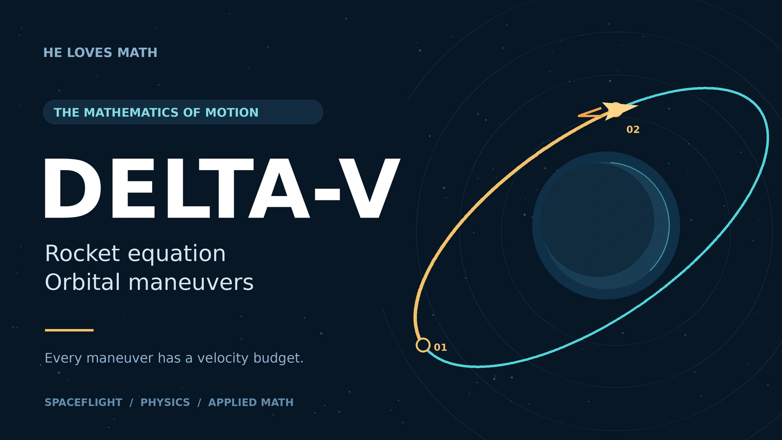
Delta-V Calculator
Estimate rocket propulsion capability, work backward to propellant, or compare idealized orbital maneuvers. Choose from eight calculation modes, then use the formulas, solved examples and self-check questions to understand the result.
Calculate Delta-V
Select a mode, enter rocket or orbital parameters, then review the delta-v, mass ratio, propellant requirement, and maneuver breakdown.
Tsiolkovsky Rocket Equation Calculator
Required Propellant and Mass Ratio Calculator
Multi-Stage Delta-V Calculator
Enter one stage per line as: stage name, Isp(s), initial mass, final mass, losses(m/s)
Hohmann Transfer Delta-V Calculator
Plane Change and Combined Burn Delta-V Calculator
Escape Injection / C3 Delta-V Calculator
Mission Delta-V Budget Calculator
Enter one maneuver per line as: maneuver name, delta-v in m/s
Delta-V Unit Converter
Delta-V Chart and Calculation Details
What is delta-v?
Delta-v, written Δv, means a change in velocity. Velocity has both magnitude and direction: a spacecraft can spend propellant to turn even when its speed stays the same. A maneuver budget normally adds the magnitudes of the required velocity changes.
There are two different questions to ask. Capability: how much ideal delta-v can a propulsion system deliver from its masses and effective exhaust velocity? Requirement: how much delta-v does a particular maneuver need under a stated orbital model? The calculator separates those questions so you can compare like with like.
The result is not a travel distance, an altitude, or necessarily a final speed relative to Earth. Gravity changes velocity while a spacecraft coasts, without consuming propellant. The rocket equation describes propulsion; the Hohmann and escape models describe particular impulsive maneuvers. Neither alone simulates a complete flight.
Choose a mode and check the inputs
- Rocket Equation: enter Isp in seconds or effective exhaust velocity in m/s, then initial and final attached masses in the same selected unit. An optional loss allowance is subtracted from ideal capability.
- Required Propellant: enter useful maneuver delta-v plus a separate loss allowance. Both are added before solving for the initial mass and consumed propellant.
- Multi-Stage: enter name, Isp, initial mass, final mass, losses on each line. Masses are always kg and losses m/s in this mode. A comma separates fields; do not put commas inside a stage name or a number.
- Hohmann Transfer: select the central body and enter two circular orbit radii measured from its center. The model adds the positive magnitudes of two burns, in either direction.
- Plane Change: choose equal-speed or combined speed-and-direction change. Enter the angle between the velocity vectors, between 0° and 180°.
- Escape Injection: start from a circular parking orbit. Enter its center-based radius and the desired excess speed far from the central body.
- Mission Budget: give each maneuver a name and a non-negative delta-v in m/s, then apply a margin. An optional propellant estimate needs both a positive Isp and final mass.
- Unit Converter: convert a velocity-change magnitude. An optional positive Isp adds a single-burn mass-ratio estimate.
The selected output unit and precision apply to the active mode. Reset restores that mode’s original example inputs; global output preferences remain selected. Editing inputs clears the old result until you calculate again. A rejected row is identified rather than silently omitted.
Use physically meaningful inputs. The two-body orbit equations do not check body surfaces, atmospheres, terrain or collision constraints. A positive radius is mathematically accepted even if it is inside a real body. Custom μ is always in m³/s². If your source gives km³/s², multiply by 10⁹.
Delta-v formulas and units
Use natural logarithms (ln), not base-10 logarithms. Match every velocity unit before adding terms, and use dimensionless mass ratios.
Ideal rocket delta-v: Δv = vₑ ln(m₀ / mf)
Loss-adjusted balance: Δvnet = Δvideal − losses
Isp is in seconds, g₀ in m/s², and vₑ in m/s. The conventional g₀ is 9.80665 m/s²; it is a reference used to express Isp, not the local gravitational acceleration during the burn.
Mass ratio MR = exp(D / vₑ)
Initial mass m₀ = mf × MR
Propellant mp = mf × [exp(D / vₑ) − 1]
Propellant fraction = mp / m₀ = 1 − 1/MR
mf includes everything still attached after the modeled burn. It is not automatically the empty rocket mass or just the payload. The inverse formulas assume constant effective exhaust velocity and the specified final mass.
Circular speed vc = √(μ/r)
Transfer speed vt = √[μ(2/r − 1/a)]
Burn 1 = |vt₁ − vc₁|
Burn 2 = |vc₂ − vt₂|
Total ideal Δv = Burn 1 + Burn 2
μ is the central body’s gravitational parameter. In SI calculations μ is in m³/s² and r and a are in metres. Absolute values keep maneuver costs positive for both raising and lowering transfers.
Combined vector change: Δv = √(v₁² + v₂² − 2v₁v₂ cos θ)
Escape injection: Δv = √(2μ/r + v∞²) − √(μ/r)
Characteristic energy: C3 = v∞²
The calculator accepts angles in degrees and converts them internally. C3 has velocity-squared units: v∞ in km/s gives C3 in km²/s². Budgets add burn magnitudes and multiply the sum by (1 + margin/100).
Rocket equation, mass ratio and final mass
Conservation of momentum gives the ideal rocket equation when effective exhaust velocity is constant. Increasing Isp increases delta-v in direct proportion for the same mass ratio. Increasing the mass ratio increases delta-v logarithmically: equal additive increases in mass ratio give progressively smaller gains.
Doubling the mass ratio adds vₑ ln(2); it does not generally double the existing delta-v. For example, with Isp = 300 s, going from mass ratio 2 to 4 adds about 2,039 m/s. Going from 4 to 8 adds the same amount, but requires another doubling of initial mass relative to final mass.

Count all attached mass. Structure, engines, payload, remaining stages, reserved propellant and other equipment belong in the final mass if still attached after this burn. Consumed propellant is m₀ − mf. Jettisoned structure between burns is accounted for separately.
Losses here are a user-supplied accounting allowance. They are not calculated from drag, thrust history, gravity, steering or burn duration. If the entered losses exceed the ideal delta-v, the negative balance means a shortfall; it is not negative usable capability or a prediction of backward motion. Equal masses yield zero ideal propulsion delta-v.
Multi-stage rockets: account for each burn
The stage calculator sums Ispᵢg₀ ln(m₀ᵢ/mfᵢ) minus the losses for each row. Include the entire attached stack in both masses for that burn. In particular, the lower stage must accelerate the upper stages and payload while they are attached.
A stage can finish at 8,000 kg, discard 2,000 kg of empty structure, and leave 6,000 kg at the start of the next burn. The mass discarded in between does not generate rocket delta-v by itself in this simple model. Its benefit is that later propulsion has less dead mass to accelerate.
The displayed stage mass-ratio product is a product of burn ratios. It is generally different from liftoff mass divided by final mass when staging drops structure. Propellant mass sums only the mass consumed within each entered burn. The tool does not infer missing jettison events or ensure that separately entered rows form a complete physical vehicle.
Use a separate row when the effective exhaust velocity or burn mass interval changes. A single “average Isp” applied to the complete liftoff-to-payload ratio can conceal important stage differences. The worked two-stage example below shows the accounting explicitly.
Hohmann transfers: radius, direction and assumptions
A Hohmann model joins two circular, coplanar orbits around one central body with a half-ellipse and two instantaneous burns. For an outward transfer, the first prograde burn raises the opposite apsis; the second prograde burn circularizes at the larger radius. For an inward transfer, both burns are retrograde. The calculator reports positive burn costs in either direction.

Radius is measured from the center. Convert altitude using r = body radius + altitude. As a teaching example, an altitude of 500 km above a spherical body of radius 6,371 km corresponds to r = 6,871 km. Entering 500 km would place the modeled point inside that body.
The two burns need not equal the difference between initial and final circular speeds. During the coast, gravity continuously changes the spacecraft’s speed and direction. A higher circular orbit has lower circular speed, yet the outward Hohmann maneuver uses prograde impulses to raise orbital energy.
This model excludes atmosphere, finite-duration burns, non-spherical gravity, plane changes, other bodies, launch windows and rendezvous phasing. It is not always the best transfer among every possible strategy; other transfer families or objectives can change the tradeoff. Equal radii require no ideal Hohmann burn, although a supplied allowance is still added.
Plane changes and combined burns
For two equal-speed velocity vectors separated by θ, the triangle formed by their difference gives Δv = 2v sin(θ/2). The angle inside the sine is half the change in direction. At a fixed angle, doubling the speed doubles the ideal cost.
An orbital plane change must occur at an intersection of the relevant planes. Use the actual angle between the velocity directions at the burn. Subtracting two listed inclinations is not sufficient when the ascending nodes differ. The familiar equal-speed plane-change relation applies directly to appropriate tangential velocities, such as circular orbits or an apsis; arbitrary locations on eccentric orbits require fuller geometry.
The combined mode allows the initial and target speed magnitudes to differ. It takes the magnitude of the vector difference, not a scalar sum of a separate speed change and plane change. Numerically, the implementation uses a stable equivalent form to avoid losing very small turns through subtraction of nearly equal squares.
The accepted direction angle is 0° through 180°. At 0°, the combined cost is |v₂ − v₁|. At 180° and equal speed it is 2v. A zero-speed vector is allowed as a mathematical limit, but that alone is not a circular-orbit plane-change scenario.
Escape injection and C3
Escape mode begins in an existing circular parking orbit. A prograde tangential impulse raises the speed from vc = √(μ/r) to the departure periapsis speed √(2μ/r + v∞²). The difference is the required ideal injection burn. The tool adds a separate non-negative loss allowance if entered.
v∞ is the speed remaining far away in the two-body model, not the burn size and not the speed at periapsis. C3 = v∞² measures the departure energy parameter. A value of 2.5 km/s therefore gives C3 = 6.25 km²/s².
At v∞ = 0 the result is the parabolic escape limit. The vehicle is already moving at circular speed, so it does not need to add the entire local escape speed. Reaching the selected parking orbit is outside this calculation. Choosing a higher starting orbit does not by itself establish the lowest total mission cost.
Build a mission delta-v budget
List every separate burn as a positive magnitude. Add losses only if they are not already inside that line item, then apply the chosen percentage margin. A negative margin is not accepted. The default entries are illustrative allowances, not a validated mission, a launch quote or a destination guarantee.
Margins do not recover omitted maneuvers. Check whether launch, orbit insertion, disposal, course corrections and other phases belong to the specific problem. Do not add an ideal burn and a published “total including losses” for that same burn, because that counts it twice.
The optional propellant estimate treats the entire budget as one equivalent constant-Isp burn on an unchanged vehicle. It assumes a fixed final mass, no refueling and no intermediate mass jettison. If the mission uses different engines or staging, calculate the appropriate phases individually. A single Isp attached to a multistage launch-to-landing budget is not a vehicle-sizing model.
Eight worked delta-v examples
These original examples use g₀ = 9.80665 m/s² and, for Earth, μ = 3.986004418 × 10¹⁴ m³/s². Keep extra digits during calculation; round the final result.
Example 1: How much delta-v can a rocket provide?
A spacecraft has Isp=320 s, initial mass 12,000 kg and final attached mass 4,000 kg. Allow 200 m/s for modeled losses.
- Convert specific impulse to effective exhaust velocity: ve=320×9.80665=3,138.128 m/s.
- Find the mass ratio: MR=12,000/4,000=3. The logarithm must be the natural logarithm: ln(3)=1.09861229.
- Ideal delta-v is 3,138.128×ln(3)=3,447.59 m/s.
- The loss-adjusted balance is 3,447.59−200=3,247.59 m/s, or 3.24759 km/s.
- Propellant consumed is 12,000−4,000=8,000 kg. Propellant fraction is 8,000/12,000=66.67% of initial mass.
The 4,000 kg is all mass still attached after this burn, including payload and any reserves. Entering payload alone would overstate performance. The result is an idealized propulsion capability, not a prediction of speed relative to the ground.
Example 2: Work backward from a required maneuver
A vehicle needs 1,800 m/s of useful maneuvering and a separate 150 m/s loss allowance. Isp is 300 s, and the mass after the burn must be 800 kg.
First add requirements: Δvrequired=1,800+150=1,950 m/s. Here ve=300×9.80665=2,941.995 m/s.
MR=exp(1,950/2,941.995)=1.94024749.
m0=800×1.94024749=1,552.20 kg.
mp=m0−mf=1,552.20−800=752.20 kg.
The propellant fraction is 48.46%. The extra allowance increases the required ideal delta-v before exponentiation; subtracting it would incorrectly reduce the propellant requirement. This answer assumes the specified final mass already includes the tanks, engine, payload and remaining reserves.
Example 3: Stages and discarded structure
Consider two sequential burns. Stage 1 has Isp=300 s and takes the attached stack from 20,000 kg to 8,000 kg, with 150 m/s of losses. The vehicle then discards 2,000 kg of spent structure. Stage 2 begins at 6,000 kg, finishes at 2,000 kg, has Isp=340 s and loses 50 m/s.
Stage 1: Δv1=300×9.80665×ln(20,000/8,000)−150=2,545.72 m/s.
Stage 2: Δv2=340×9.80665×ln(6,000/2,000)−50=3,613.06 m/s.
Total: Δv1+Δv2=6,158.78 m/s.
The two burns consume 12,000+4,000=16,000 kg of propellant. The separate 2,000 kg discarded between burns is not burned propellant. The burn mass-ratio product is 2.5×3=7.5, while the starting-to-final stack ratio is 20,000/2,000=10. These differ because mass was jettisoned between burns. This is why stage-by-stage accounting matters.
Example 4: Raise a circular orbit with two Hohmann burns
Transfer between Earth-centered circular radii of 7,000 km and 14,000 km. Both orbits are in the same plane. These are distances from Earth's center, not altitudes above the surface.
The transfer ellipse has a=(7,000+14,000)/2=10,500 km. Using consistent SI units:
- Initial circular speed: vc1=√(μ/r1)=7,546.05 m/s
- Transfer speed at the first burn: vt1=√[μ(2/r1−1/a)]=8,713.43 m/s
- First burn magnitude: |vt1−vc1|=1,167.38 m/s
- Transfer speed at the second burn: vt2=4,356.72 m/s
- Final circular speed: vc2=5,335.87 m/s
- Second burn magnitude: |vc2−vt2|=979.15 m/s
Total ideal transfer delta-v is 2,146.53 m/s. Both burns are prograde, even though the final circular speed is lower than the starting speed: the spacecraft slows while coasting outward as kinetic energy becomes gravitational potential energy. The reverse transfer has the same total burn magnitude, with the burn order reversed and both burns retrograde. Neither direction includes launch, plane change or rendezvous timing.
Example 5: Change direction, or combine direction and speed
For a pure 5° plane change at a tangential orbital speed of 7,500 m/s:
Δv=2×7,500×sin(5°/2)=654.29 m/s.
The sine receives half the angle, 2.5°, not the whole 5°. The result is a cost even though speed stays unchanged, because velocity includes direction.
For a separate combined-vector example, let v1=1,000 m/s, v2=1,600 m/s and the angle between the velocity vectors be 30°. The required single impulse is:
Δv=√[1,000²+1,600²−2×1,000×1,600×cos(30°)]=888.10 m/s.
Changing direction at 1,000 m/s first and then increasing speed would cost 2×1,000×sin(15°)+600=1,117.64 m/s in two ideal burns at the same point. The combined impulse saves 229.54 m/s in this vector comparison. A real orbital maneuver also needs a location where the intended velocity vectors and trajectories are compatible.
Example 6: Escape from a parking orbit
A spacecraft starts in a circular Earth orbit of radius 6,771 km and needs hyperbolic excess speed v∞=2.5 km/s. Convert v∞ to 2,500 m/s before combining it with SI orbit speeds.
vc=√(μ/r)=7,672.60 m/s.
vesc=√(2μ/r)=10,850.69 m/s.
vp=√(vesc²+v∞²)=11,134.97 m/s.
Δvinjection=vp−vc=3,462.37 m/s.
C3=(2.5 km/s)²=6.25 km²/s². C3 is not 6.25 km/s, and v∞ is not the burn size. The vehicle is already traveling at circular speed before the burn. This ideal tangential injection does not include reaching the parking orbit. If v∞=0, the same relation gives the limiting parabolic-escape burn.
Example 7: Build a budget before estimating propellant
A teaching mission has three separate maneuver allowances: 120 m/s for orbit adjustment, 650 m/s for transfer and 80 m/s for corrections.
Base budget=120+650+80=850 m/s.
15% margin=0.15×850=127.5 m/s.
Design total=850+127.5=977.5 m/s.
If one unchanged vehicle performs every burn at Isp=320 s and ends at 900 kg, an ideal equivalent estimate is:
MR=exp[977.5/(320×9.80665)]=1.36546009.
mp=900×(MR−1)=328.91 kg.
Do not use this single-Isp mass estimate for a mission that drops stages, uses engines with different Isp, or refuels along the way. Use the relevant phase masses and engine performance instead. A percentage margin is an allowance chosen by the user, not a replacement for identifying omitted maneuvers or losses.
Example 8: Convert units without changing the maneuver
For Δv=2.4 km/s:
- m/s: 2.4×1,000=2,400 m/s
- ft/s: 2,400/0.3048=7,874.02 ft/s
- mph: 2,400/0.44704=5,368.65 mph
- km/h: 2,400×3.6=8,640 km/h
These are four descriptions of the same velocity change. A conversion changes the number and unit together; it does not change propellant demand. Radius and μ units must be consistent separately: km³/s² converts to m³/s² by multiplying by one billion, not one thousand.
Practice: calculate, then reveal the explanation
Use the stated units and the ideal models above. Try each question before opening its answer.
Question 1
An engine has effective exhaust velocity 3,000 m/s and a mass ratio of 4. What is its ideal delta-v?
Show answer 1
Δv=3,000 ln(4)=4,158.88 m/s. The mass ratio is dimensionless. Using log10 would give a different, incorrect result because the rocket equation comes from the natural logarithm.
Question 2
A vehicle must deliver 1,500 m/s, its effective exhaust velocity is 3,000 m/s, and its final mass is 500 kg. How much propellant is needed in the ideal single-burn model?
Show answer 2
MR=exp(1,500/3,000)=exp(0.5)=1.64872127. Initial mass is 824.36 kg, so propellant is 324.36 kg. Multiplying the final mass directly by Δv/ve would miss the exponential dependence.
Question 3
A spacecraft is at altitude 500 km above a spherical body of radius 6,371 km. What radius should be entered in an orbital calculator?
Show answer 3
r=6,371+500=6,871 km. Entering 500 km treats the craft as 500 km from the center, which is inside this body. The example adopts a stated spherical radius; it does not resolve geodetic/equatorial distinctions.
Question 4
A pure plane change of 60° occurs at tangential speed 2,000 m/s. Find its delta-v. What if the speed were halved?
Show answer 4
Δv=2×2,000×sin(30°)=2,000 m/s. At 1,000 m/s it costs 1,000 m/s. For a fixed angle this ideal cost is directly proportional to speed, which motivates planning plane changes at suitable lower-speed locations.
Question 5
Maneuvers cost 200, 500 and 50 m/s. Add a 20% margin.
Show answer 5
The base is 750 m/s, the margin is 150 m/s, and total is 900 m/s. Margin multiplies the entire base budget by 1.20; it is not an extra 20 m/s.
Question 6
A circular orbit has speed 7,000 m/s. Ignoring losses, how much additional speed is needed to just escape with zero excess speed?
Show answer 6
Local escape speed is √2×7,000=9,899.49 m/s, so the burn is 9,899.49−7,000=2,899.49 m/s. Escape speed and the required departure burn are different quantities because the vehicle already has orbital speed.
Question 7
A stage ends its burn at 8,000 kg, drops 2,000 kg of structure, and the next stage starts burning. What starting mass belongs to the next stage? Is the discarded structure counted as consumed propellant?
Show answer 7
The next stage starts at 6,000 kg. The dropped structure is a separate mass change, not burned propellant. It lowers the mass that the next burn must accelerate, which is the performance benefit of staging.
Question 8
A Hohmann transfer is reversed, with the same two circular coplanar radii and no losses. Does the total delta-v become negative?
Show answer 8
No. The impulses switch to retrograde, and their order reverses, but the sum of their positive magnitudes is unchanged. Signed velocity changes indicate direction; propellant budgeting uses their magnitudes.
Common delta-v mistakes
- Speed versus velocity: changing direction costs delta-v even at the same speed. Orbital speed is not the same quantity as launch propulsion delta-v.
- Altitude versus radius: add the body radius before using center-based orbital formulas. Positive numbers can still describe physically impossible orbits.
- Local gravity versus standard gravity: keep the standard Isp reference g₀ on the Moon or Mars. Change the orbital μ preset for orbital calculations.
- Incomplete final mass: include all still-attached equipment and reserves. “Dry mass” and “final burn mass” are not interchangeable in every problem.
- Logarithm or unit errors: use ln, convert km/s to m/s when needed, and convert μ from km³/s² to m³/s² with a factor of one billion.
- Negative burn budgets: prograde/retrograde indicate direction. Add positive magnitudes for propellant budgets; a negative loss-adjusted rocket balance is a shortfall.
- Double-counted losses: do not add the same allowance twice. The budget tool does not infer what a supplied number already includes.
- One number for an entire real mission: finite burns, thrust limits, atmospheres, gravity fields and operational constraints require models beyond this educational page.
Delta-v FAQs
What does this Delta-V Calculator do?
It covers rocket capability, required propellant, stage sums, Hohmann transfers, pure or combined vector changes, escape injection, mission budgets and unit conversion. Each mode uses a stated idealized model.
What is delta-v?
It is a change in velocity or a propulsion/maneuver budget expressed in velocity units. A turn can need delta-v even when the speed remains unchanged.
What is the rocket equation?
The ideal relation is Δv = Isp g₀ ln(m₀/mf) = vₑ ln(m₀/mf), for constant effective exhaust velocity. The masses describe the same burn and include everything attached.
What is mass ratio?
For one burn it is m₀/mf, a dimensionless ratio of starting to ending attached mass. In a staged calculation, the product of burn ratios can differ from the full vehicle’s starting-to-final ratio because structure is discarded.
Why is staging useful?
Discarding spent tanks and engines reduces the mass that later burns must accelerate. Enter the attached upper stages and payload in each burn’s mass accounting.
Why are plane changes expensive?
Their cost depends on the angle between velocity vectors and the speed at the maneuver. In the equal-speed ideal model it is 2v sin(θ/2). The maneuver geometry still has to be physically possible.
Can this calculator be used for real mission design?
No. It is for education and preliminary mathematical exploration. Flight decisions require validated propulsion and trajectory tools, full constraints and qualified engineering review.
Should I change g₀ to lunar gravity?
No, not for Isp stated in standard seconds. Keep g₀ = 9.80665 m/s². The central-body μ preset is the separate parameter used by the orbital modes.
Can a Hohmann transfer go inward?
Yes. The two impulses become retrograde. The calculator adds their positive magnitudes, so the reversed ideal transfer has the same total cost between the same circular coplanar radii.
Why does the result say shortfall?
The loss allowance is larger than the ideal rocket capability. The negative balance describes a deficit under the entered assumptions, not usable negative delta-v.
Constants, precision and related study
For continuity with the tool’s existing Earth examples, presets use Earth μ = 3.986004418 × 10¹⁴, Sun μ = 1.32712440018 × 10²⁰, and the rounded educational Mars value 4.282837 × 10¹³ m³/s². The lunar preset is updated to JPL’s DE440 value, 4.902800118 × 10¹² m³/s². These are model conventions, not claims of unlimited physical precision.
Exact conversions used here include 1 ft = 0.3048 m, 1 international mile = 1609.344 m, 1 lb = 0.45359237 kg, and 1 tonne = 1000 kg. Displaying five decimal places does not improve uncertain inputs. Values outside the supported numerical range produce a clear error rather than an apparently valid infinite mass.
Continue with the orbital velocity calculator, escape velocity calculator, or length converter for related mathematical quantities. Review each model’s assumptions separately.
Educational model limitations
This page is for mathematical learning. It does not evaluate a flight trajectory, launch safety, collision avoidance, vehicle certification or operational feasibility. Examples and default budgets are illustrative. Use qualified engineering review and validated mission-analysis software for real spacecraft decisions.
Sources & References
Primary references consulted on 6 October 2026. Worked examples, practice problems and artwork on this page are original calculations and illustrations.
- NASA Glenn: Ideal Rocket Equation — Conservation-of-momentum model, effective exhaust velocity and the ideal mass-ratio relation.
- NASA Glenn: Specific Impulse — Definition of Isp and its relation to effective exhaust velocity.
- NIST SP 811: Appendix B.9 conversion factors — Standard acceleration reference and unit conversions.
- NASA/JPL Basics of Space Flight: Chapter 4, Trajectories — Transfer-orbit geometry and the context of idealized trajectories.
- FAA: Maneuvering in Space (PDF) — Educational derivations and discussion of orbit and plane-change maneuvers.
- NASA Ames: Trajectory Browser User Guide — Characteristic energy C3, excess velocity and two-body departure assumptions.
- JPL Solar System Dynamics: Astrodynamic Parameters — GM/μ values and ephemeris conventions, including the DE440 lunar parameter.