
Try each part before reading the solution. Show the statistical method as well as the calculation, check conditions when needed, and state conclusions in the problem’s context. A calculator is allowed throughout. Keep unrounded probabilities in later calculations; round final answers sensibly and include units.
This guide covers the single publicly released 2026 AP Statistics free-response set on AP Central, checked October 11, 2026. It contains no secure multiple-choice questions. The 90-minute section contains six questions; the suggested pacing is 65 minutes for Questions 1–5 and 25 minutes for Question 6. Each question receives a rubric score from 0 to 4; those rubric scores should not be confused with the exam’s weighted scoring. The original HeLovesMath solutions below were independently checked against the official scoring guidelines.
For additional practice, browse our AP Statistics past-question collection or review the statistics and probability formula sheet.
Goat Weights: Summaries, Spread, and Shape
The official rubric evaluates A, B, and C as whole parts; C(i) and C(ii) contribute to the same part. Three essentially correct parts earn 4 points.
Part A
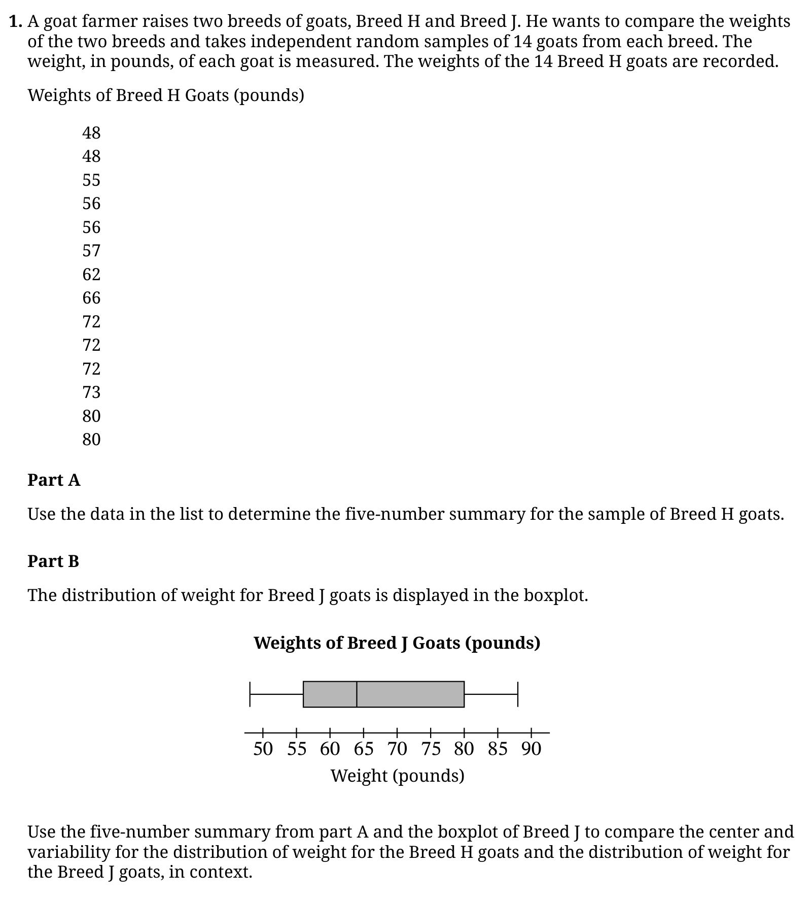
- The 14 weights are already in increasing order. The first and last observations give a minimum of 48 pounds and a maximum of 80 pounds.
- With an even number of observations, average the two central observations, in positions 7 and 8: pounds.
- The lower half is 48, 48, 55, 56, 56, 57, 62. Its middle value, the fourth observation, is 56, so the first quartile is 56 pounds.
- The upper half is 66, 72, 72, 72, 73, 80, 80. Its middle value is 72, so the third quartile is 72 pounds.
- Report the summary in the order minimum, first quartile, median, third quartile, maximum.
Credit check: Label the five quantities or put exactly five numbers in the standard increasing order. Do not substitute the sample mean for the median.
Part B
- Read the median line in the Breed J boxplot at approximately 64 pounds. The median for Breed H is 64 pounds, so the two breeds have approximately the same sample median weight.
- For Breed H, pounds. For Breed J, the left and right edges of the box are approximately 56 and 80 pounds, so pounds.
- As a second comparison of spread, pounds, while the Breed J whiskers extend from approximately 48 to 88 pounds, giving pounds.
- Both measures indicate more variability in the sampled Breed J goat weights. An explicit comparison matters more than simply listing the summaries.
Credit check: Compare medians and either IQRs or ranges in the context of the two goat breeds and their weights. A boxplot does not provide enough information to calculate either sample mean exactly.
Part C(i)
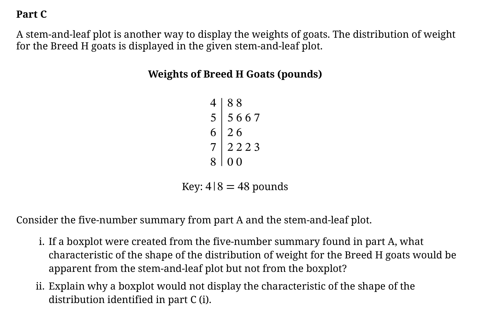
- The stem-and-leaf plot shows four observations in the 50s and four in the 70s, with only two in the 60s between them.
- These concentrations form two peaks or clusters, one in the 50-pound range and one in the 70-pound range.
- This two-peaked shape is not visible from the five-number summary alone.
Credit check: The characteristic is bimodality. A list of repeated numerical values or a statement of symmetry alone does not identify the missing shape feature.
Part C(ii)
- A boxplot locates the minimum, quartiles, median, and maximum. It does not show each goat weight or how often each value occurs.
- Consequently, the boxplot conceals how observations are concentrated within the sections between its summary values.
- Different data sets can have the same five-number summary while having different numbers of peaks. Thus a roughly symmetric-looking boxplot need not describe a unimodal distribution.
Credit check: Connect the missing peaks to the information the boxplot suppresses. Do not claim that a symmetric boxplot establishes a normal distribution.
Rosebush Experiment: Design and Significance
The official rubric evaluates A, B, and C as whole parts. The three identifications in A are evaluated together; three essentially correct parts earn 4 points.
Part A(i)
- A treatment is a specific experimental condition imposed on an experimental unit.
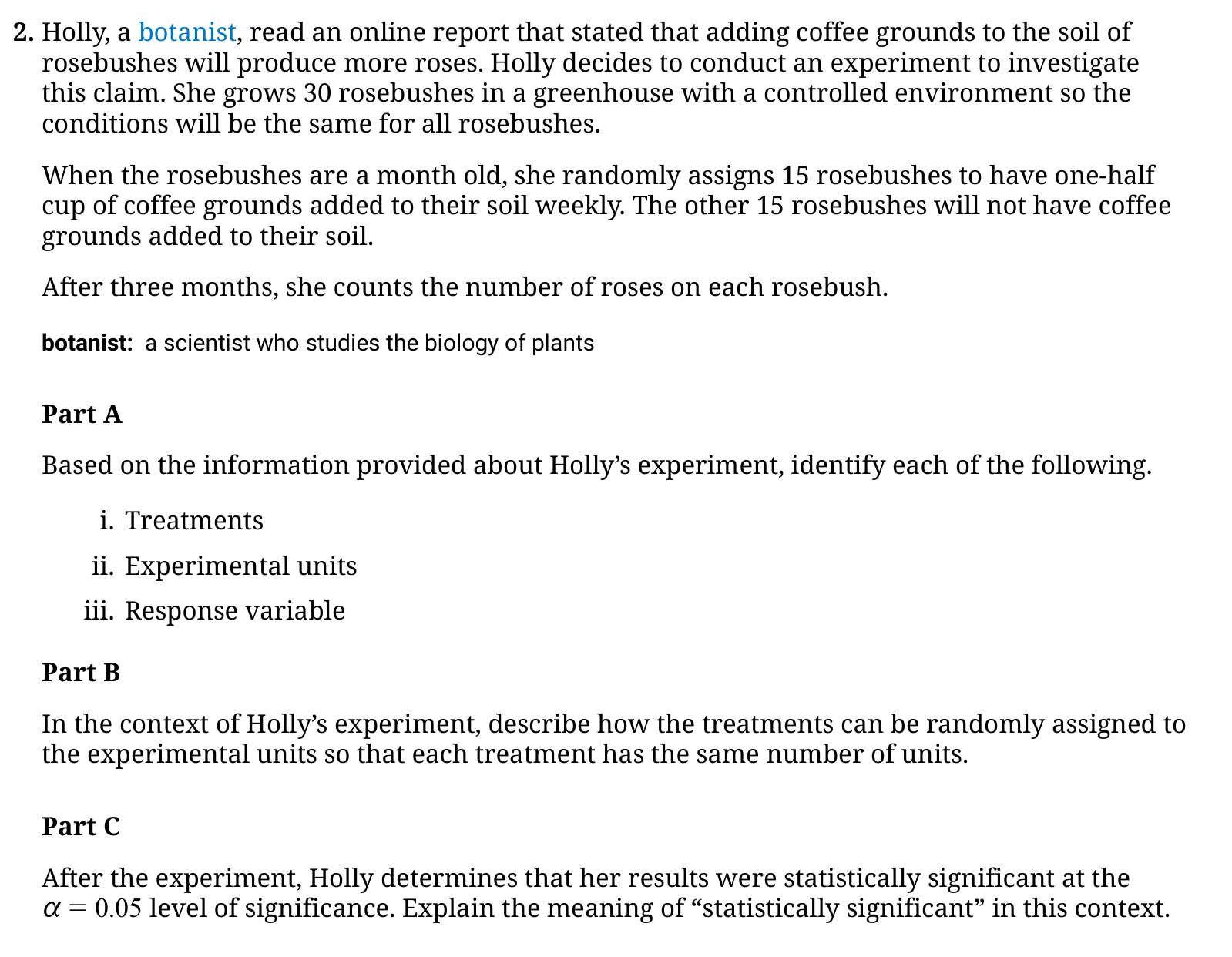
- Holly imposes two conditions: adding one-half cup of coffee grounds to a rosebush's soil each week, or adding no coffee grounds.
- The greenhouse conditions are held constant; they are not separate treatments being compared.
Credit check: Identify both conditions, including the no-coffee control treatment.
Part A(ii)
- Experimental units are the objects to which the researcher randomly assigns treatments.
- Holly assigns a soil treatment to each of her 30 rosebushes, so each individual rosebush is one experimental unit.
Credit check: Distinguish a rosebush, which receives a treatment, from a rose, which is counted as part of the response.
Part A(iii)
- The response variable is the measurement collected from each experimental unit after the treatments have been applied.
- Holly counts how many roses are on each rosebush after three months.
Credit check: State the individual rose count, not the treatment indicator or the mean count across a treatment group. The group means are summaries of the response variable.
Part B
- Label the 30 rosebushes with the distinct numbers 1 through 30. Prepare 30 otherwise identical slips of paper, one labeled with each number.
- Place the slips in a container and mix them thoroughly. Draw 15 slips without replacement.
- Assign the 15 rosebushes whose labels were drawn to receive one-half cup of coffee grounds in their soil weekly.
- Assign the remaining 15 rosebushes to receive no coffee grounds.
- Because the slips are thoroughly mixed and equally likely to be drawn, every set of 15 rosebushes has the same chance to receive coffee grounds. Drawing without replacement guarantees exactly 15 different bushes in each group.
Credit check: Give an implementable random process, connect selected labels to treatments, and guarantee 15 units in each group. Flipping coins independently need not give equal group sizes; stopping coin flips when one group fills does not make all balanced assignments equally likely.
Part C
- Start with the no-effect assumption: adding coffee grounds does not affect the mean number of roses per rosebush.
- Even under that assumption, random assignment can produce different sample mean rose counts in the two groups.
- Statistical significance at means the observed difference is sufficiently unusual under the no-effect assumption: the probability of a difference at least as extreme as the one observed, arising through random assignment alone, is below 0.05.
- Thus the experiment supplies evidence of an effect of the coffee-grounds treatment on rose production. The statement of significance by itself does not quantify the size or practical importance of that effect.
Credit check: Mention the difference between the groups, random chance, and the number of roses. A p-value is not the probability that the no-effect hypothesis is true, nor the probability that the result was caused by chance.
Song Durations: Normal, Binomial, and Geometric Models
The official rubric evaluates A, B, C, and D as whole parts; C(i) and C(ii) are combined. Each essentially correct part contributes 1 point, with partial-credit and holistic rules for intermediate totals.
Part A
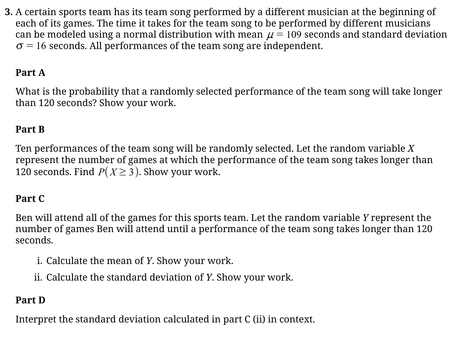
- Let be the length of a randomly selected performance, in seconds. The stated model is normal with population mean seconds and population standard deviation seconds.
- Standardize the boundary: .
- The requested event is a right tail: .
- Evaluating gives . Equivalently, use a normal cumulative-probability calculation with lower bound 120, upper bound , mean 109, and standard deviation 16.
Credit check: Show the normal model and parameters, the boundary 120, and the upper-tail direction. The performance time is continuous, so do not replace the boundary by 121 seconds.
Part B
- There are a fixed 10 performances. Each either exceeds 120 seconds or does not. The performances are independent, and each has the same success probability found in A.
- Therefore , where . Here a success means a performance longer than 120 seconds.
- At least three successes is the complement of zero, one, or two successes: .
- Calculate .
- A calculator equivalent is . Here the trial count is n = 10, p is the unrounded success probability from A, and the cumulative upper bound is 2.
Credit check: Subtract the cumulative probability through 2, not through 3. Use the exact binomial model; a normal approximation is unsuitable because the expected number of successes is only about 2.46.
Part C(i)
- Now the number of performances is not fixed in advance. Ben attends until the first performance that lasts longer than 120 seconds, counting the game with that performance.
- Because the trials are independent and each has the same success probability , has a geometric distribution on .
- For this convention, games.
- Although each observed count is a whole number, its long-run mean need not be a whole number.
Credit check: Count the successful game as part of Y. The formula (1-p)/p would count only the preceding unsuccessful games. Keep a decimal mean rather than rounding to 4 or 5.
Part C(ii)
- For the geometric count of trials through the first success, .
- Taking a square root gives .
- Substitute the probability from A: games.
Credit check: Report the standard deviation, not the variance. The units are games because Y counts games; they are not seconds.
Part D
- Imagine repeatedly restarting this process and counting games until the first team-song performance longer than 120 seconds.
- The long-run mean of those counts is approximately 4.07 games, while the standard deviation measures the typical amount by which the counts differ from their mean.
- Use the value from C(ii) as a measure of spread for these waiting-time counts, not as a spread for individual song lengths.
Credit check: Include repeated trials or the long run, variation around the mean, and the event that ends the count. A standard deviation is not a statement that every waiting time lies within 3.53 games of the mean.
Orange Fertilizers: Complete Two-Sample Inference
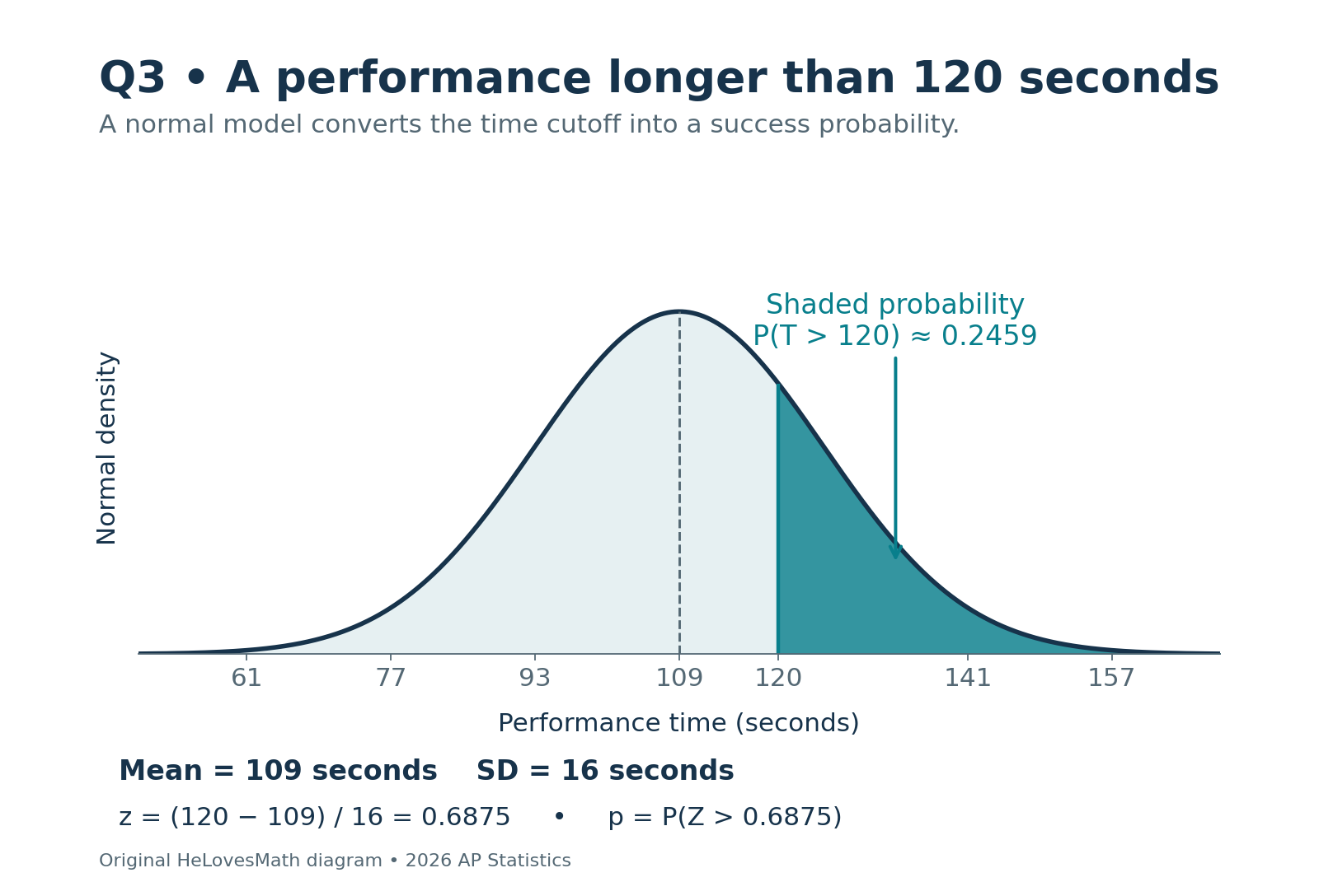
This question has no lettered subparts. The official rubric scores three sections: hypotheses and procedure; conditions and calculations; and conclusion. All three essentially correct sections earn 4 points.
Complete hypothesis test
- Define the parameters. Let be the population mean number of oranges per tree when trees similar to those in the experiment receive Brand C fertilizer. Let be the corresponding population mean under Brand N.
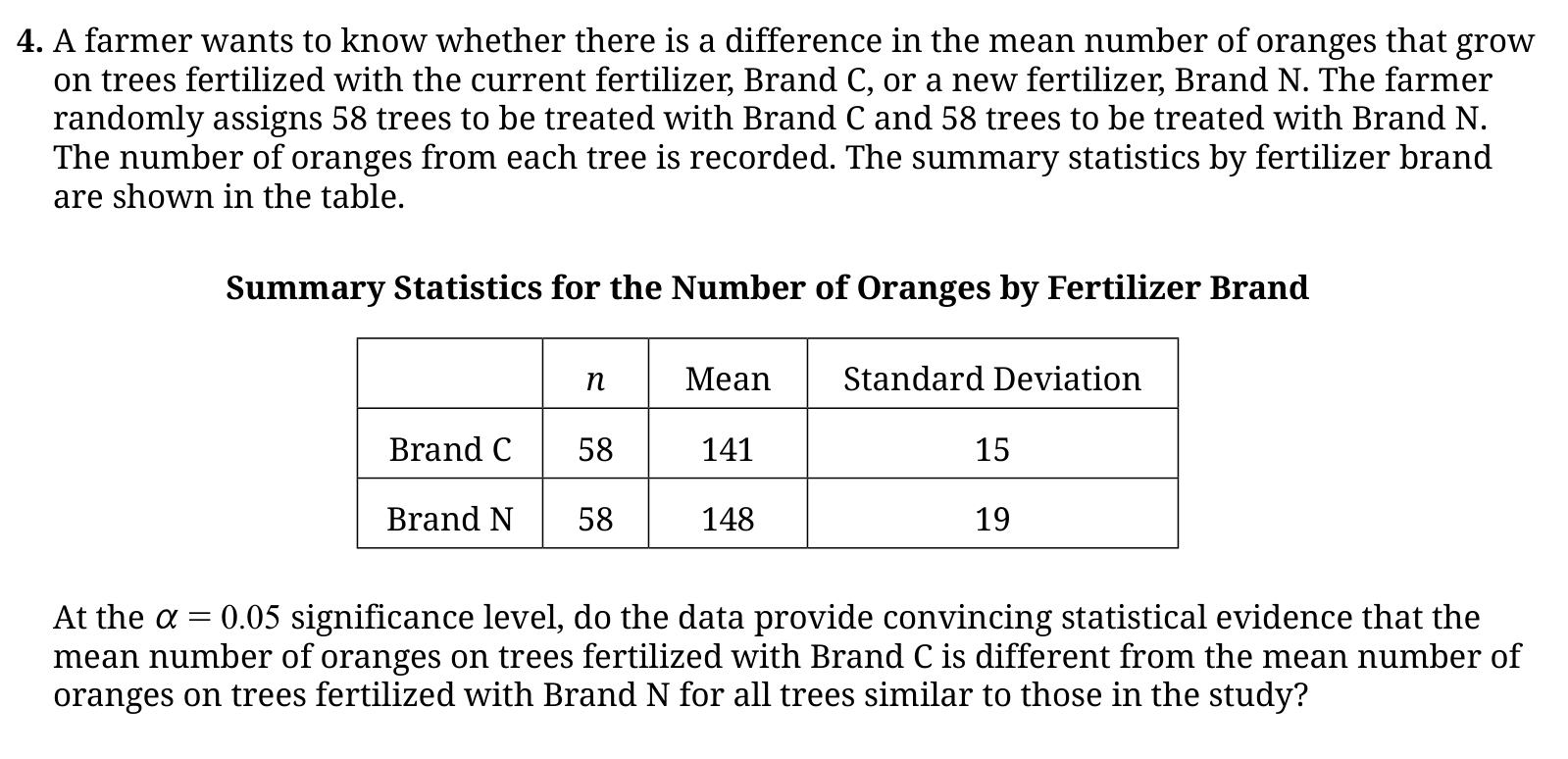
- State the hypotheses: versus . The question asks whether the means differ, so the alternative is two-sided.
- Choose an independent two-sample t-test for a difference of population means, using the unpooled/Welch standard error. The population standard deviations are unknown. These are two groups of trees, not paired measurements on the same trees.
- Check randomization: the farmer randomly assigned 58 trees to each fertilizer. This is random treatment assignment in an experiment; the question does not say the trees were a random sample.
- Check the large-sample condition: . Thus the sampling distribution of the difference in sample means is approximately normal. The usual experimental analysis treats the separate trees as independent experimental units, with no interference between treatments.
- Find the observed difference: oranges per tree.
- Estimate its standard error: oranges per tree.
- Compute the standardized statistic: .
- Let and . Welch's degrees of freedom are .
- For the two-sided alternative, . The factor of 2 accounts for a difference at least this far from 0 in either direction.
- Compare with the stated significance level: . Reject .
- Conclude in context: the data provide convincing statistical evidence that the population mean number of oranges per tree under Brand C differs from the population mean under Brand N for trees similar to those studied. The Brand N group had the larger observed sample mean, by 7 oranges per tree; the inference requested here is a difference between the treatment means.
Credit check: Give population parameters, a two-sided alternative, random assignment, both sample sizes, the t statistic and p-value, and a contextual conclusion. Do not claim random sampling, use a paired test, or require a 10% sampling check for this randomized experiment. Say there is evidence of a difference rather than that the test proves one. The official rubric also accepts the conservative df=57 calculation, which gives p about 0.032 and the same decision.
Athlete Ages: Conditional Probability, Mosaic Plots, and Census Data
The official rubric evaluates A, B, C, and D as whole parts, with the two leaf responses in A, B, and C combined within each part. Each essentially correct part contributes 1 point, with partial-credit and holistic rules for intermediate totals.
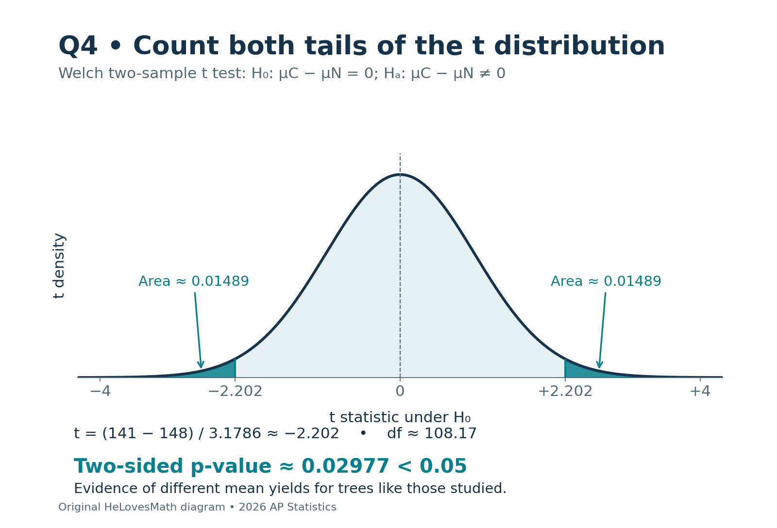
Part A(i)
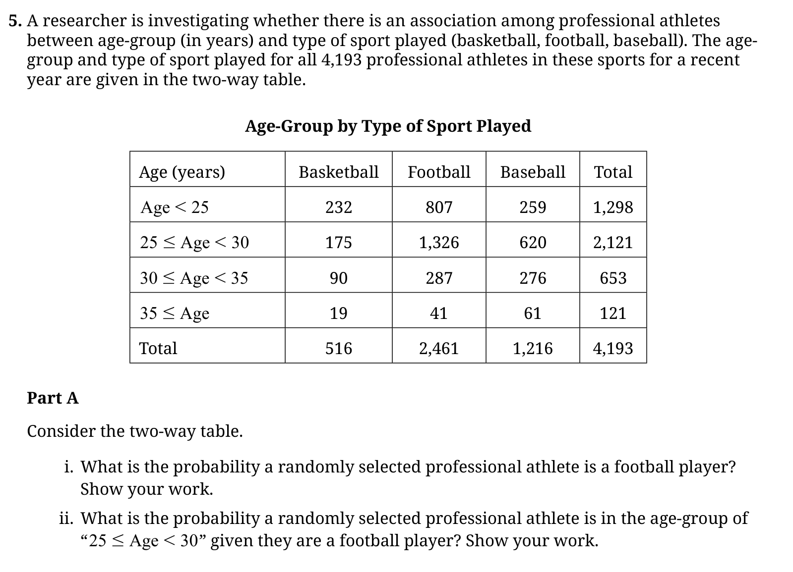
- Let F denote the event that the selected athlete plays football. The random selection is from all 4,193 athletes in the table, so 4,193 is the denominator.
- The football column contains 2,461 athletes.
- Therefore .
Credit check: Use the football column total over the grand total. This is a marginal probability, without an age restriction.
Part A(ii)
- Let F mean the athlete plays football, and let A mean the athlete is at least 25 but younger than 30 years old. The phrase given they are a football player restricts the sample space to the 2,461 football players.
- Among those football players, 1,326 are at least 25 years old and younger than 30.
- Thus .
Credit check: The denominator is the total in the conditioning group, not 4,193 and not the total number aged 25 to under 30.
Part B(i)
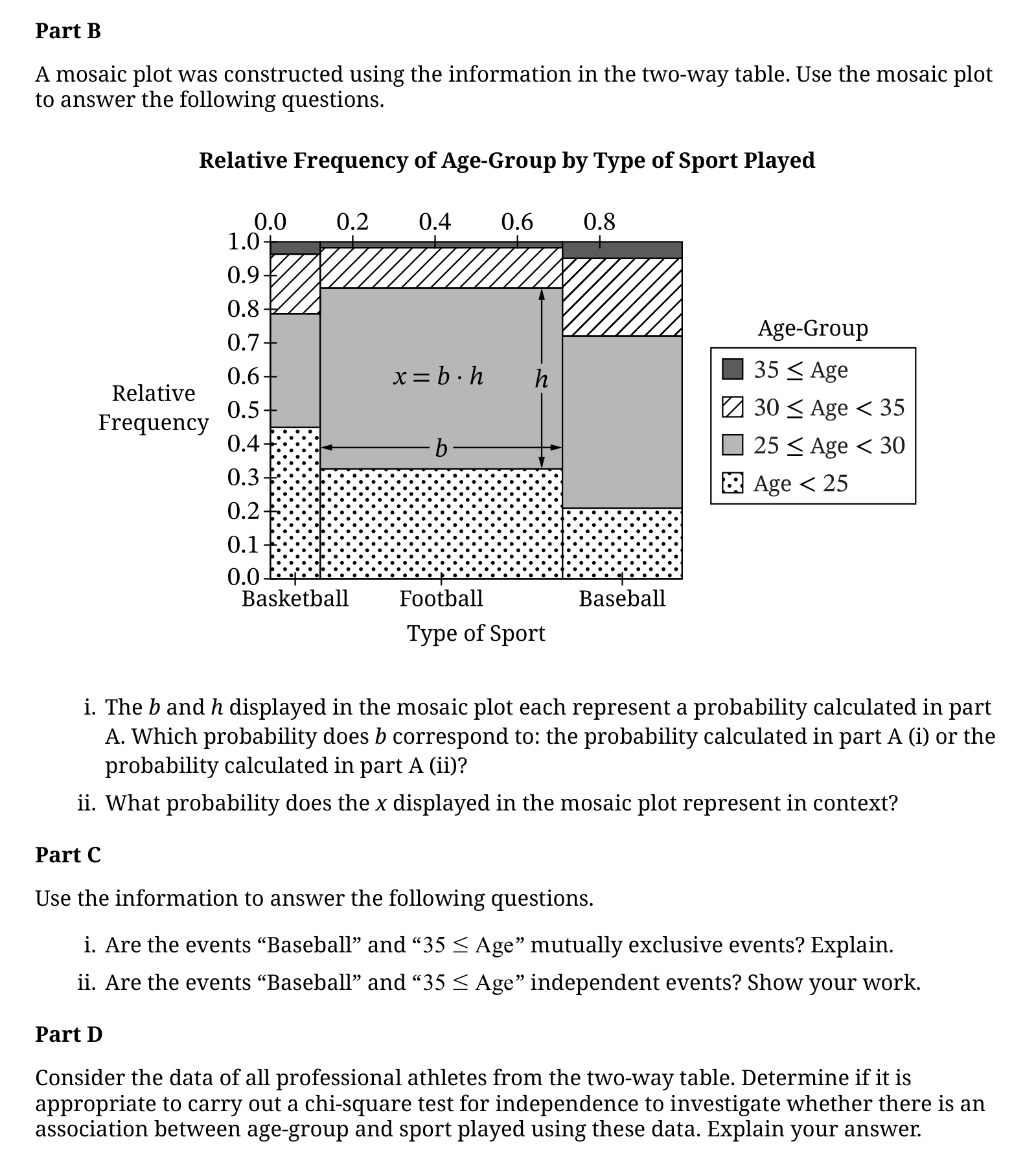
- Let F denote the event that the athlete plays football. In the mosaic plot, a sport's column width represents its share of all athletes.
- The segment labeled b spans the width of the football column.
- Therefore , the marginal probability calculated in A(i). The height h, by contrast, is the age-group proportion within the football column.
Credit check: A column width gives the marginal sport probability; an age-band height within that column gives the conditional age probability.
Part B(ii)
- Let F mean the athlete plays football, and let A mean the athlete is at least 25 but younger than 30 years old. The area of a mosaic rectangle represents the proportion of all individuals who meet both its column and row conditions.
- Here .
- Substituting gives . Simplifying gives .
Credit check: This is a joint probability for a selection from all athletes. Saying only a randomly selected football player is aged 25 to under 30 describes a conditional probability instead.
Part C(i)
- Let B mean the athlete plays baseball, and let G mean the athlete is at least 35 years old. Mutually exclusive events cannot occur for the same selected athlete.
- The table contains 61 athletes who play baseball and are at least 35 years old.
- Therefore , so their intersection is not empty.
Credit check: Explain with the overlap count or its positive probability. Mutually exclusive is a different concept from independent.
Part C(ii)
- Let B mean the athlete plays baseball, and let G mean the athlete is at least 35 years old. If the events were independent, knowing an athlete is at least 35 would not change the probability that the athlete plays baseball: .
- Among the 121 athletes aged 35 or older, 61 play baseball, so .
- Among all athletes, .
- These probabilities are different. In this population, athletes aged 35 or older are more likely to be baseball players than athletes selected without that age condition.
Credit check: Show a relevant conditional-versus-marginal comparison, or compare the joint probability with the product of the marginals. The mere existence of overlap does not establish dependence.
Part D
- A chi-square test of independence is an inferential procedure: it uses sample data to assess a possible association in a larger population.
- This table contains every athlete in the specified three professional sports for that year. It is a census of the population of interest, not a random sample from that population.
- Because the entire population is observed, there is no sampling uncertainty about its age-by-sport distribution to assess with an inferential test. Its association can be described directly using the observed proportions.
Credit check: Base the answer on the census/no-random-sampling issue. Large cell counts do not create a need for inference, and the finding of dependence in C(ii) alone is not the reason the test is inappropriate.
Baseball Regression: Relationships and Two Types of Intervals
The official rubric evaluates A, B, C, and D as whole parts; their leaf responses are combined. Each essentially correct part contributes 1 point, with partial-credit and holistic rules for intermediate totals.
Part A(i)
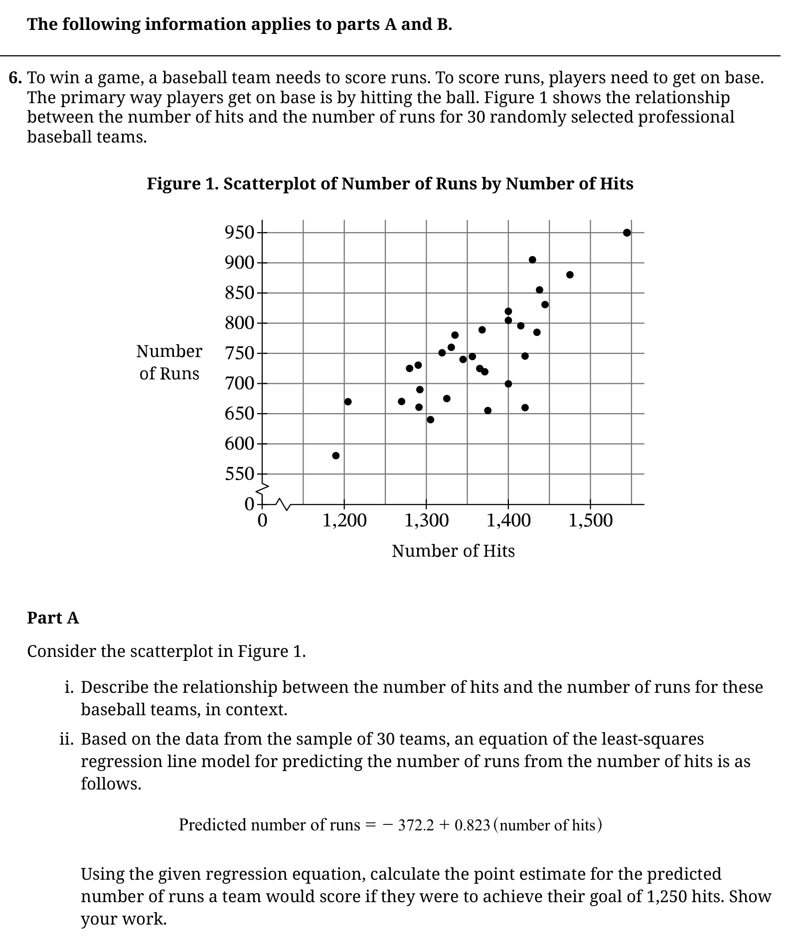
- Identify the variables: the horizontal coordinate is the number of hits by a baseball team, and the vertical coordinate is its number of runs.
- The cloud of points rises from left to right, giving a positive association: teams with more hits tend to score more runs.
- The overall pattern is reasonably close to a straight line, so a linear form is appropriate.
- There is noticeable scatter, but the upward pattern is clear; moderately strong describes its strength.
Credit check: Include direction, form, strength, and both variables in context. Describe association rather than claiming that the scatterplot by itself demonstrates causation.
Part A(ii)
- Use the provided fitted line .
- Substitute the goal of 1,250 hits: .
- Calculate , then subtract 372.2 to obtain .
- Keep 656.55 as the point estimate for the later interval calculations. A model's predicted count need not itself be an integer.
Credit check: Show the substitution into the regression equation. Keep the decimal prediction for C rather than accumulating error by rounding early.
Part B(i)
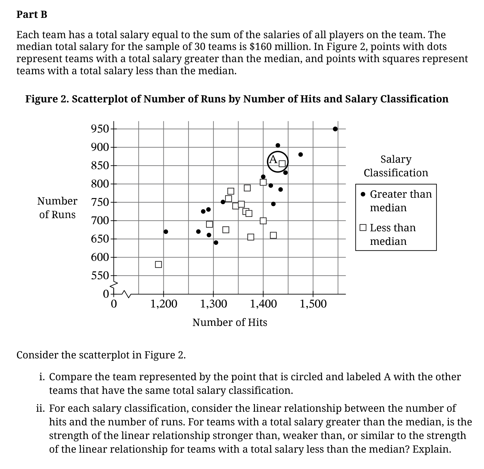
- The circled point A is a square. According to the key, that means its team's total salary is below the sample median of 160 million dollars.
- Compare A only with the other squares, as the question asks for teams in the same salary classification.
- A is farther to the right and higher than every other square, so it has both the largest number of hits and the largest number of runs within that below-median-salary group.
Credit check: Mention both hits and runs, and compare with the correct salary group. Point A is not the highest-run or highest-hit team among all 30 teams.
Part B(ii)
- Examine how tightly each group's points follow its own straight-line pattern.
- The dots, representing teams with total salaries above the median, cluster more tightly around an increasing linear trend.
- The squares, representing teams below the median salary, are more widely scattered around their increasing trend.
- Less scatter around a line corresponds to a stronger linear association. This comparison concerns strength, not simply the steepness of the trend or which teams have larger counts.
Credit check: Support the comparison using closeness to a linear pattern. A larger slope, higher runs, or a larger range alone does not imply a stronger correlation.
Part C(i)
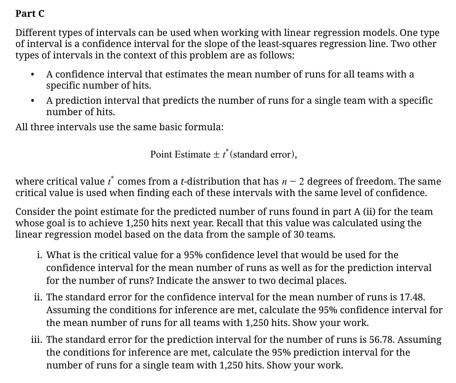
- For these regression intervals, the question specifies . With 30 teams, .
- A central 95% interval leaves 2.5% in each tail, so use the 97.5th percentile of the t distribution.
- , which rounds to 2.05 at the requested two decimal places.
Credit check: Use n-2 degrees of freedom and a two-sided 95% critical value. The normal value 1.96 and the one-sided 95% t critical value are not the requested values.
Part C(ii)
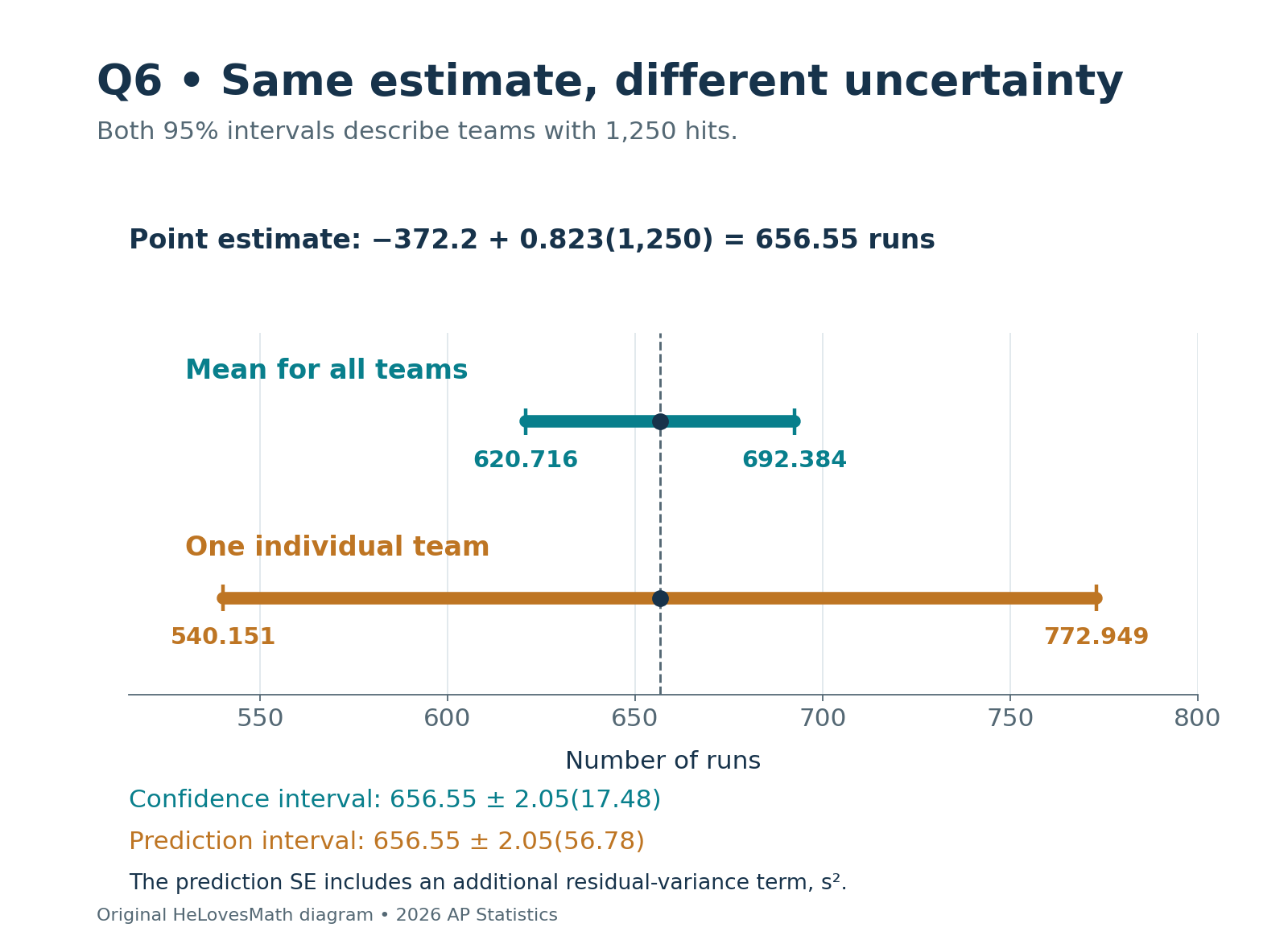
- The point estimate at 1,250 hits is runs, and the given standard error for estimating the mean response is 17.48 runs.
- Use .
- The margin of error is runs.
- The endpoints are and runs.
- We are 95% confident that the mean number of runs for all teams with 1,250 hits lies between approximately 620.72 and 692.38 runs, assuming the stated inference conditions hold.
Credit check: Use the mean-response standard error 17.48. This interval estimates a mean; it does not describe where 95% of individual teams fall. Keeping the unrounded t critical value gives (620.74, 692.36), which the official rubric also accepts.
Part C(iii)
- The same point estimate, runs, centers the prediction interval for a single team with 1,250 hits.
- Use the larger individual-prediction standard error, 56.78 runs: .
- The margin of error is runs.
- The endpoints are and runs.
- We predict, with 95% confidence, that a single team with 1,250 hits will score between approximately 540.15 and 772.95 runs, assuming the stated conditions. Over repeated applications of this procedure, about 95% of such prediction intervals would contain the corresponding individual team's run count.
Credit check: Use 56.78 for the prediction standard error and keep the same center and critical value. Keeping the unrounded t critical value gives (540.24, 772.86), also accepted by the official rubric.
Part D(i)
- A single observation may lie far above or below the population mean. An average combines several observations, so unusually high and low values tend to offset one another.
- As a result, sample means fluctuate less from sample to sample than individual observations fluctuate from observation to observation.
- For independent observations with population standard deviation , the standard deviation of a sample mean is , which is less than when .
Credit check: Explain the effect of averaging. Merely quoting the two numerical standard errors from C does not explain why distributions of means are less variable.
Part D(ii)
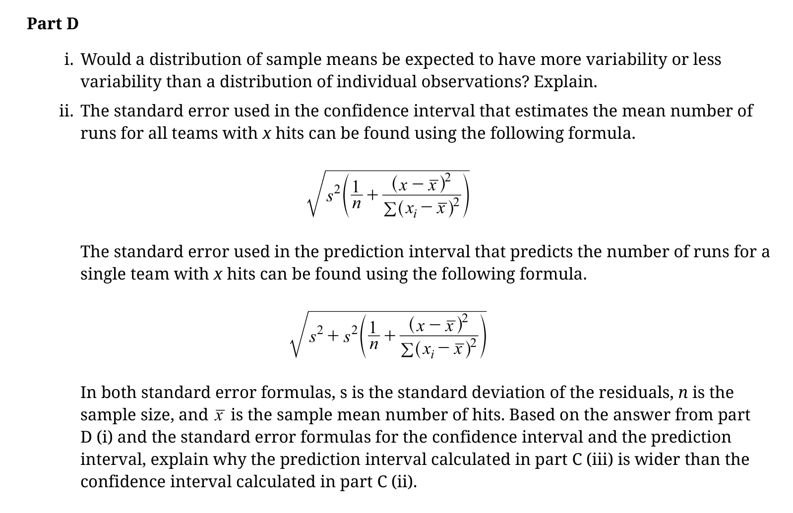
- Write the mean-response standard error as .
- The prediction standard error includes an additional residual-variance term: .
- The confidence interval for the mean response allows for uncertainty in estimating that mean. The prediction interval must additionally allow for the random variation of one individual team's runs around the mean response.
- Here , so . This matches D(i): individual outcomes vary more than averages.
- Both intervals have the same point estimate and positive critical value . Since their widths are , the larger prediction standard error produces the larger margin of error and wider interval.
Credit check: Connect the extra s-squared term to individual variation and then to interval width. Both intervals have the same confidence level, sample size, center, and critical value; those features do not explain the difference in widths.
Sources & References
Official question images: © 2026 College Board. Source pages are identified beneath each image. Solutions, explanatory diagrams and feature artwork are original HeLovesMath materials. AP and Advanced Placement are registered trademarks of College Board. This page is not affiliated with or endorsed by College Board.
- College Board: AP Statistics past exam questions — official release index, checked October 11, 2026.
- 2026 AP Statistics Free-Response Questions — 13-page official public PDF; Questions 1–6 appear on pages 3–13.
- 2026 AP Statistics Scoring Guidelines — 35-page official rubric used to check every response.
The official release index linked one unnumbered 2026 free-response set and its scoring guidelines, with no separate 2026 question erratum linked at the source check.