
Try each part before reading its solution. Questions 1–2 require a graphing calculator in radian mode; Questions 3–6 do not allow a calculator. Write the mathematical setup even when a calculator gives the number. Keep unrounded values in your calculations and give final decimal answers to three places unless the question says otherwise.
This guide covers the single released 2026 BC free-response set linked on AP Central, checked October 11, 2026. It is not a complete exam and contains no unreleased multiple-choice questions. Questions 1–2 form Section II Part A (30 minutes); Questions 3–6 form Part B (60 minutes). Each question is worth 9 points. The explanations are original HeLovesMath work, checked against the official scoring guidelines.
For more practice, browse our AP Calculus BC past-exam collection.
Bird arrivals: rates, accumulated change, and the Intermediate Value Theorem
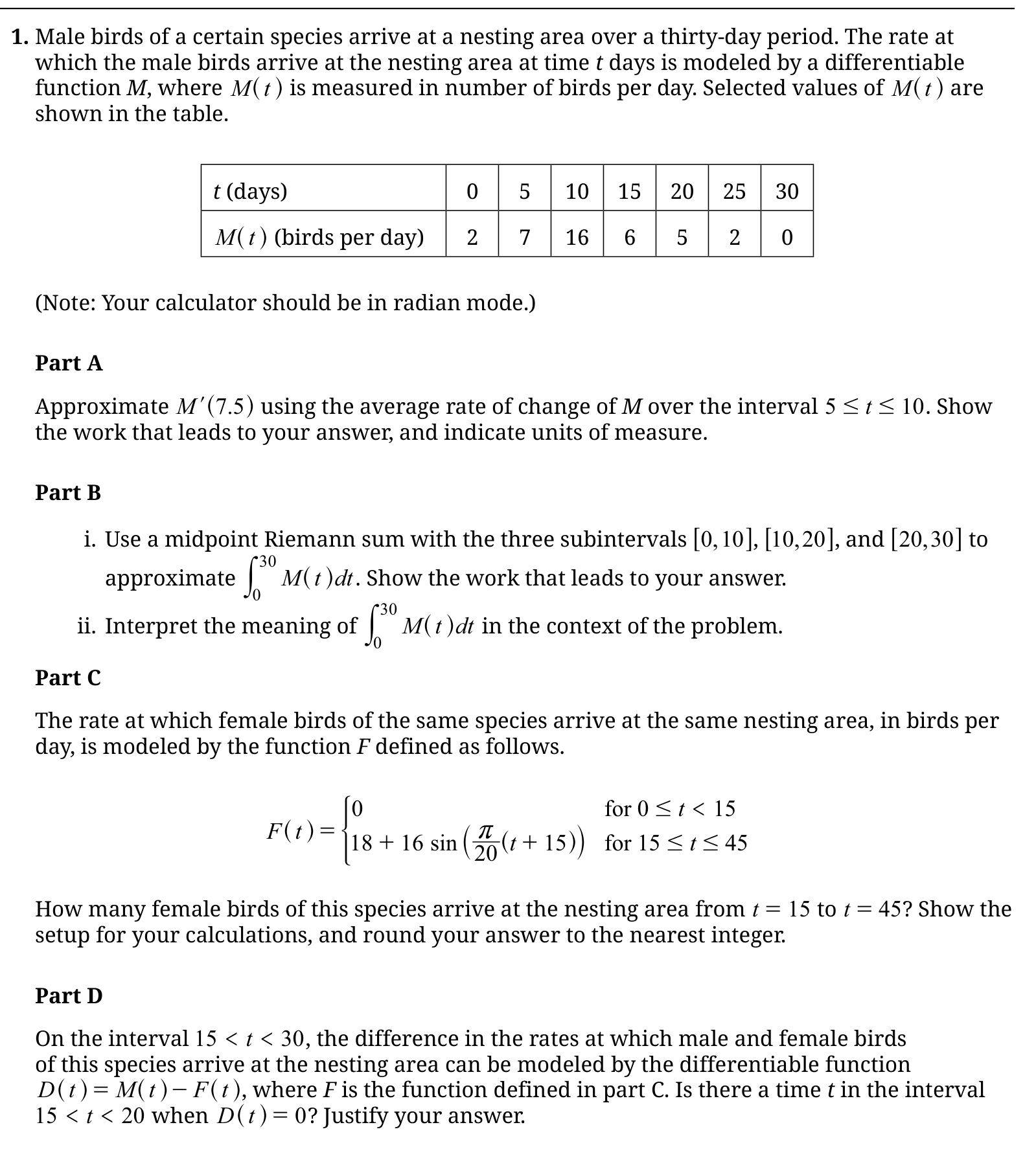
Part A
- Approximate the instantaneous rate of change at the midpoint with the secant slope across : .
- Substitute the table values and : .
- The numerator measures a change in birds per day, and the denominator is measured in days. Therefore the derivative is measured in birds per day per day, or birds per day squared.
Credit check: A derivative of an arrival rate measures how fast that rate changes. Dividing birds per day by days produces birds per day squared.
Part B(i)
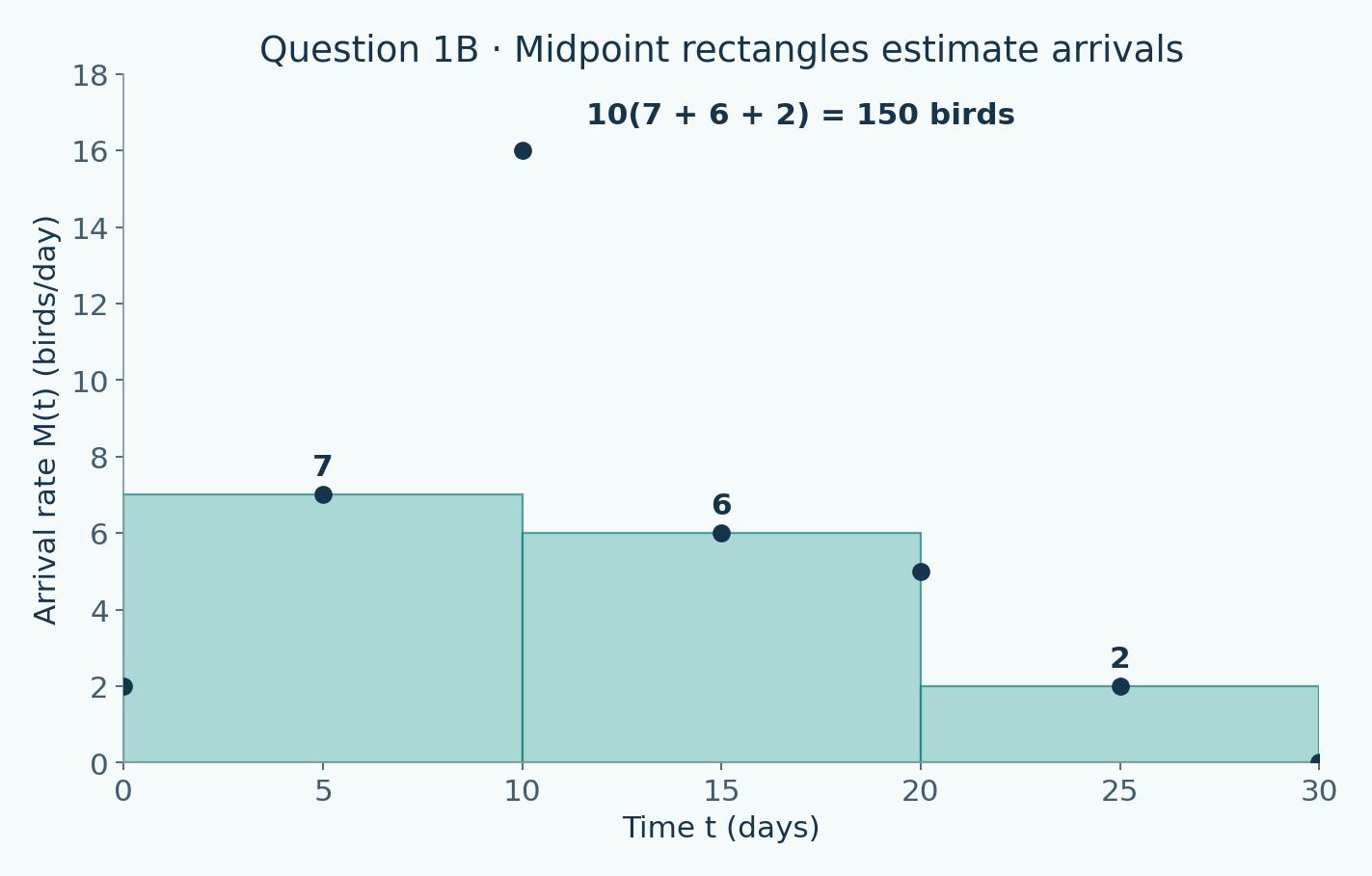
- Each requested subinterval has width days. Their midpoints are , , and .
- Use the arrival rate at each midpoint as the height of its rectangle: .
- Substitute and add: . Multiplying birds per day by days gives birds.
Credit check: Locate each midpoint before looking up its rate. The three rectangle heights are the values at days 5, 15, and 25.
Part B(ii)
- gives the rate at which male birds arrive, so integrating this rate adds up arrivals over time.
- The limits and select the entire thirty-day arrival period. Thus the integral represents the number of male birds of this species that arrive at the nesting area from day through day .
Credit check: An arrival rate integrated over time gives a total count. Include the population and the time interval in your interpretation.
Part C
- An arrival rate accumulates to a total through integration. On , use .
- Set up the total number of female arrivals as .
- A calculator in radian mode gives . Alternatively, an antiderivative is , so the exact integral is .
- Round the final total to the nearest integer, as requested: female birds.
Credit check: Integrate the rate rather than evaluating it at the endpoints. Keep your calculator in radians, and round only the final total to a whole bird.
Part D
- Differentiability implies continuity, so is continuous on its given interval. For the endpoint argument, is continuous and the sine branch of is continuous from through , so also gives a continuous extension of to .
- At the left endpoint, , so .
- At the right endpoint, . Thus .
- Because is continuous on and lies strictly between and , the Intermediate Value Theorem guarantees some with . At that time, the male and female arrival rates are equal.
Credit check: Opposite signs guarantee a zero only when continuity is established. The Intermediate Value Theorem proves existence, but it does not identify a unique time.
Polar curves: area, tangent slopes, radial extrema, and average distance
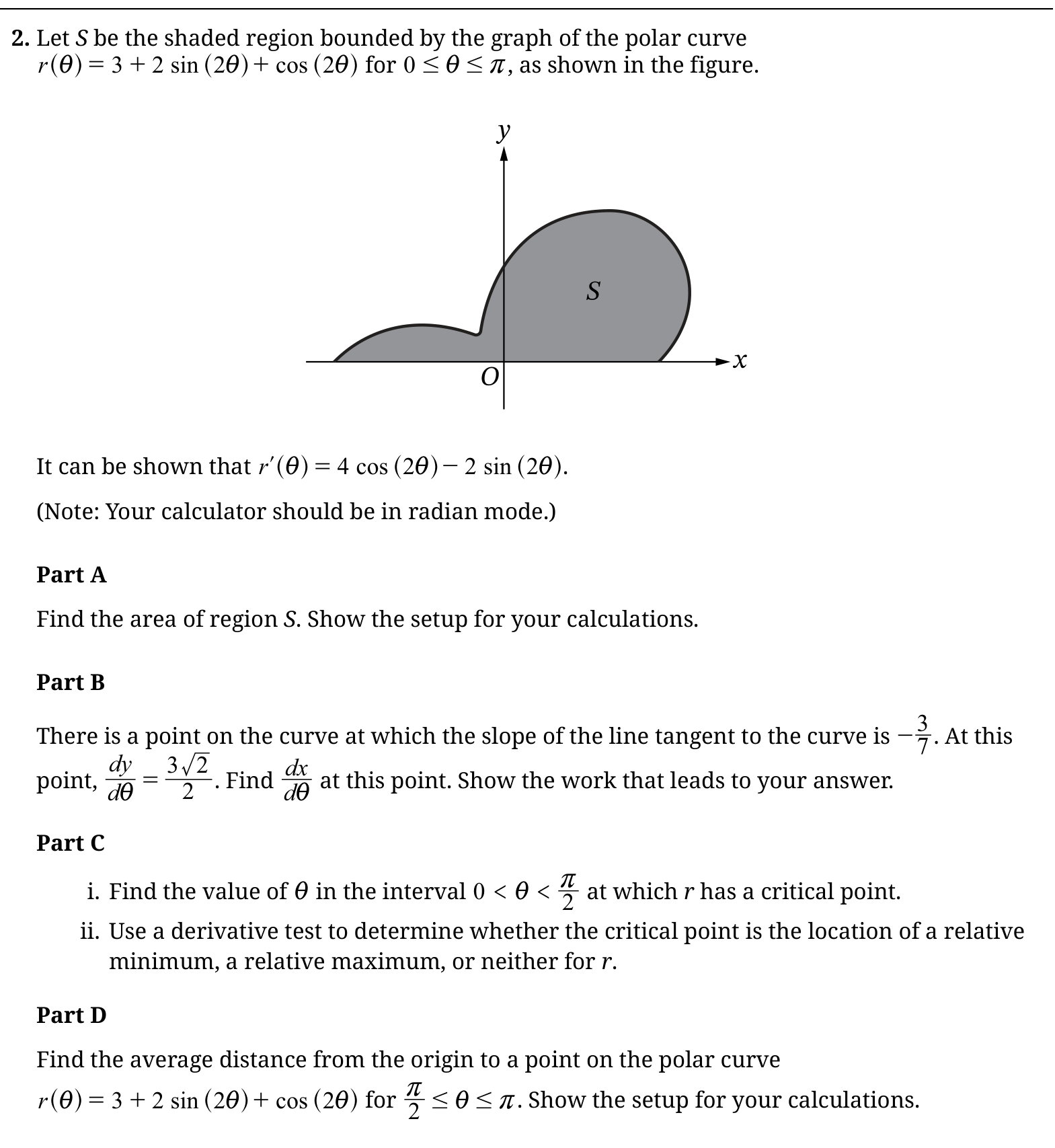
Part A
- For a polar curve, a thin sector with angle has area approximately . Add these sectors over the stated angular interval .
- The required setup is .
- Using radian mode, numerical integration gives . Thus the area is square units to three decimal places.
- An exact check is also possible. Over , the integrals of , , and vanish, while each squared trigonometric term integrates to . Expanding the square therefore gives .
Credit check: Polar area requires both the factor and the squared radius. The angular limits are and , even though the region is not a semicircle.
Part B
- Treat and as functions of the parameter . The tangent slope satisfies .
- Use the given slope and vertical component at the specified point: .
- Solve for the horizontal component by dividing the numerator by the tangent slope: .
Credit check: The tangent slope is a ratio of two derivatives. Divide by to recover ; multiplying those two given values reverses the relationship.
Part C(i)
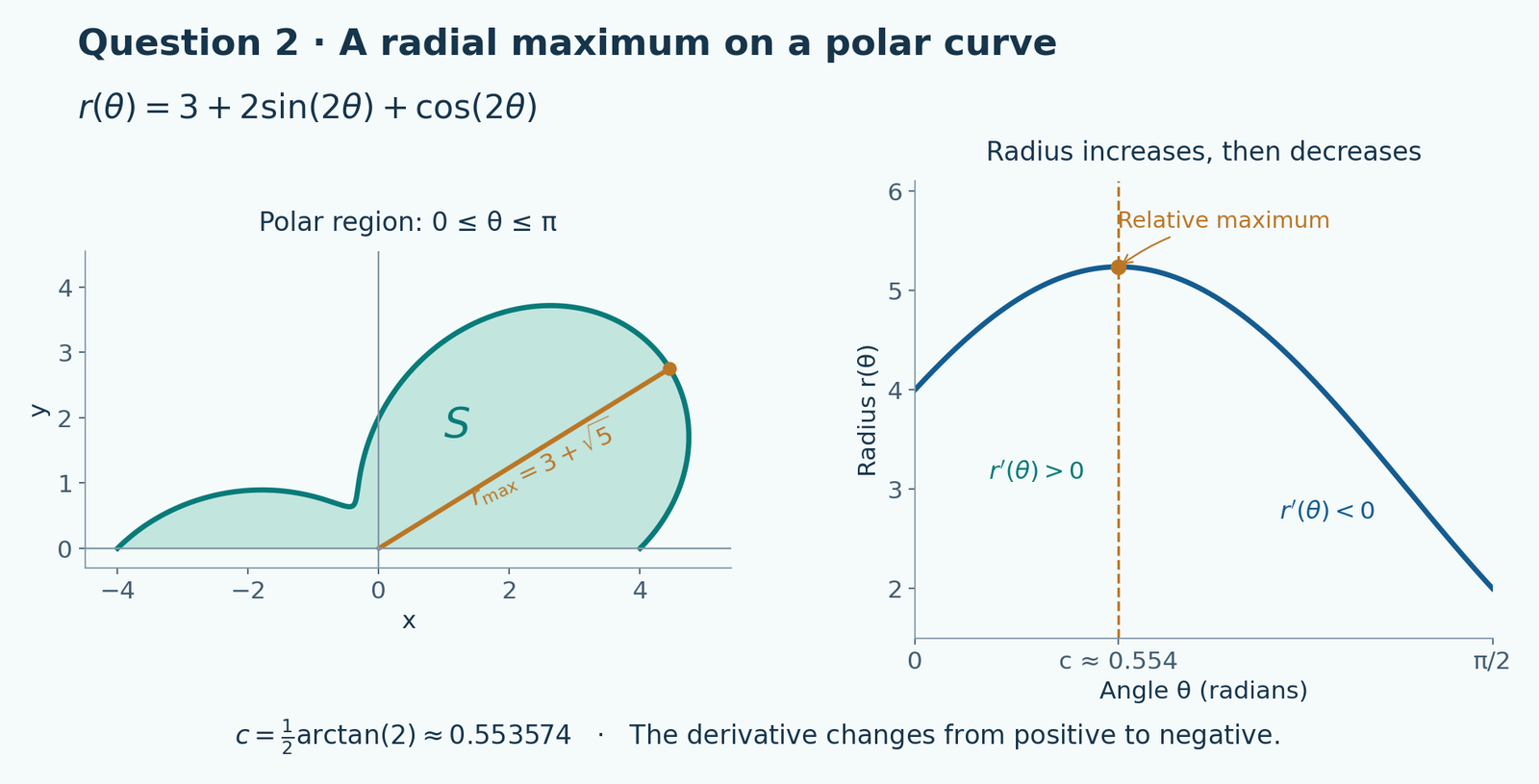
- The derivative exists everywhere, so an interior critical point occurs where this derivative equals zero.
- Set . This gives . At a solution, cannot be zero, so divide to obtain .
- Because , we have . The unique angle in this interval with tangent is . Thus radians.
Credit check: Check the interval after solving the trigonometric equation. The requested critical point belongs to the radius function , so set .
Part C(ii)
- Differentiate again: .
- At , the angle lies in the first quadrant and has tangent . Hence and .
- Substitution gives .
- Since and , the Second Derivative Test shows that has a relative maximum at . Its radius there is , although that radius is not needed to classify the point.
Credit check: A zero first derivative identifies a candidate. Complete a derivative test to classify it. Here the negative second derivative supplies the needed conclusion.
Part D
- Distance from the origin is . Here lies between and , so . Therefore the distance equals .
- Take the average value of this distance with respect to over : .
- An antiderivative is . Evaluating at the limits gives .
- Divide by the angular interval length: . The average distance is therefore units.
Credit check: An average value is an integral divided by the interval length, which here is . Average the radius itself; squaring it would produce a different quantity.
Newton's law of cooling: slope fields, tangent lines, and separation of variables
Part A
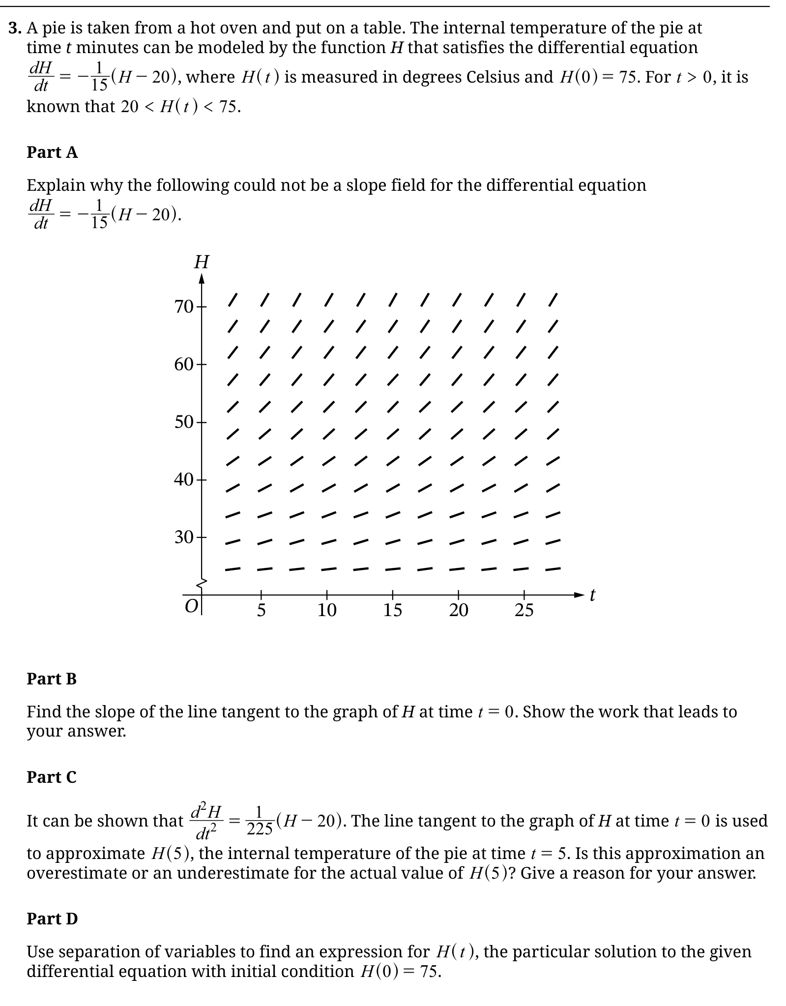
- The differential equation assigns each point the slope .
- In the displayed temperature range, , so and hence . A correct slope field would have downward-sloping line segments at these points.
- The displayed line segments instead have positive slopes. Their signs contradict the negative slopes required by the differential equation, so this cannot be its slope field.
Credit check: Compare the signs of the drawn segments with the sign required by the differential equation. Here every temperature shown is above the equilibrium temperature of 20 degrees Celsius.
Part B
- The tangent-line slope at is . Substitute the initial temperature into the differential equation.
- .
- Because measures degrees Celsius and measures minutes, this slope is in degrees Celsius per minute. The negative sign describes the pie cooling initially.
Credit check: The differential equation supplies the tangent slope directly when you substitute the initial temperature. Keep the answer as an exact fraction in this no-calculator question.
Part C
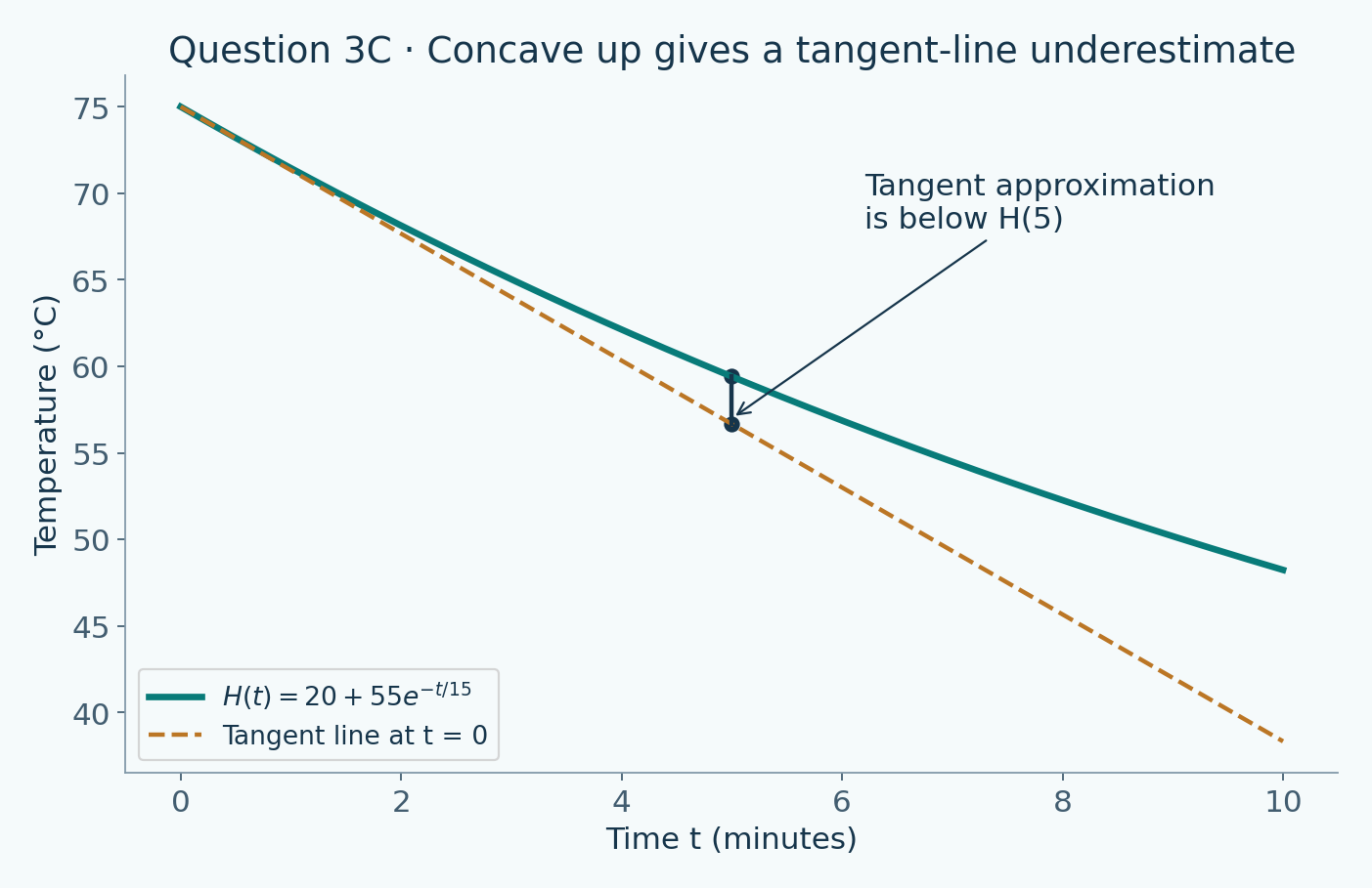
- Throughout , the given inequality makes .
- Therefore the graph of is concave up throughout the interval used for the approximation. Its tangent line at lies below the graph to the right of the tangency point.
- Consequently, evaluating that tangent line at underestimates the actual temperature .
- Optional tangent-line check: , so degrees Celsius. This value is below .
Credit check: Establish concavity throughout the interval from to . A concave-up graph stays above its tangent line, which explains the direction of the approximation error.
Part D
- Start with . Since along the solution, divide by and separate variables: .
- Integrate both sides: , giving .
- Apply : , so .
- Substitute this constant and exponentiate: implies . Because , use the positive branch: .
- Solve explicitly: . As a check, , and .
Credit check: Show separation, both integrations, an integration constant, the initial-condition substitution, and the explicit solution. A correct formula alone does not demonstrate the requested method.
Derivative graphs: concavity and absolute extrema
Part A
- Differentiate the defining equation : .
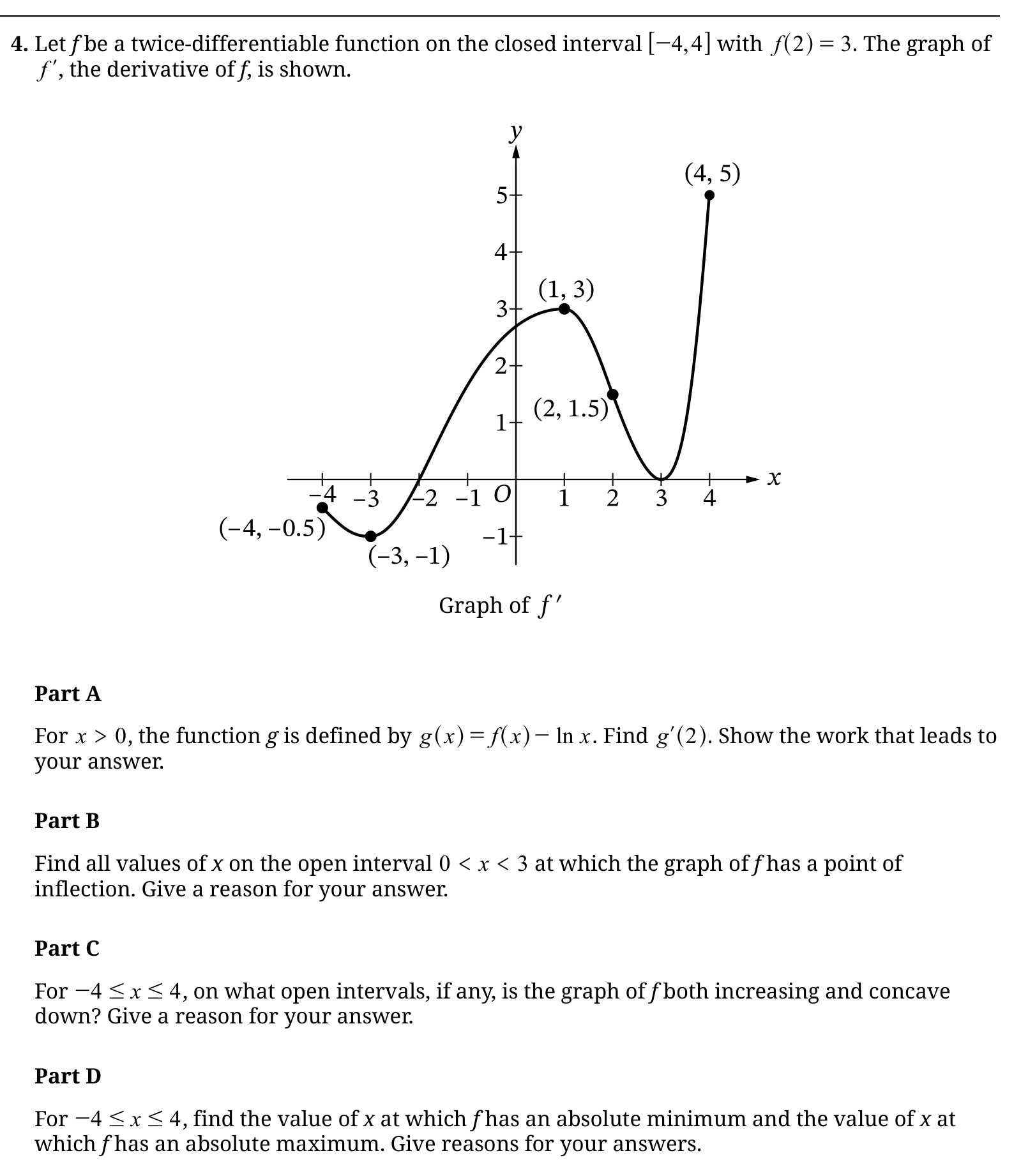
- The labeled point belongs to the graph of , so .
- Substitute into the derivative: .
Credit check: The graph gives , whereas the initial information gives a function value. Keep these quantities distinct.
Part B
- The concavity of is determined by whether its derivative is increasing or decreasing. Increasing means that is concave up; decreasing means that is concave down.
- Within the requested interval , the graph of increases on and decreases on .
- Therefore changes concavity at , and there is no other change of concavity inside .
Credit check: Name in the justification and describe its graph. The condition finds candidates for extrema of , not its inflection points.
Part C
- Two conditions must hold simultaneously: so that is increasing, and must be decreasing so that is concave down.
- The graph is above the -axis on and . It decreases on and .
- The overlap of the positive and decreasing portions is .
Credit check: The sign of the graph of controls increasing/decreasing behavior; the direction in which that graph moves controls concavity.
Part D
- To find absolute extrema on the closed interval, consider the endpoints and critical points of . From the graph, at and ; the endpoints are and .
- The derivative is negative on and positive on and . Thus decreases up to and increases afterward. The zero at does not reverse this increasing behavior, so the absolute minimum occurs at .
- The absolute maximum must therefore occur at one of the endpoints. Compare them using .
- The positive area exceeds the magnitude of the negative area. One way to make this comparison precise is to use the graph bounds: on , , so the integral there is at least ; on , , so the integral there is at least . The remaining pieces contribute nonnegative area.
- Consequently . Hence , and the absolute maximum occurs at .
Credit check: A sign change of establishes the minimum. To select the absolute maximum, also compare the two endpoint values using signed area.
Area, volume, arc length, and an improper integral
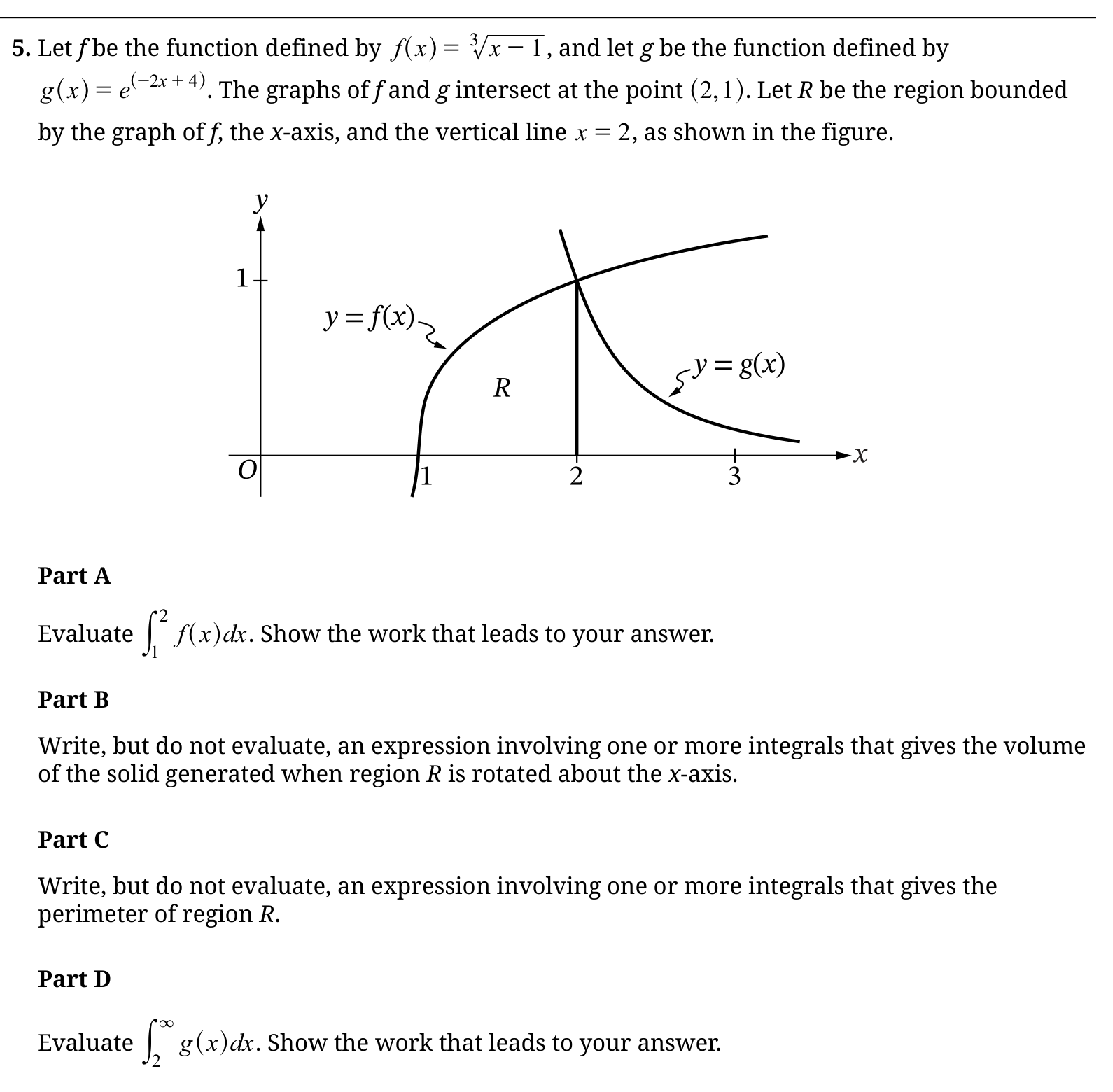
Part A
- Write the cube root as a power: . The inner function has derivative , so the power rule for integration applies directly.
- Increase the exponent by and divide by the new exponent: .
- Evaluate the endpoints: .
Credit check: Show an antiderivative and its endpoint evaluation. The cube root changes to a power when integrated.
Part B
- The region extends from the zero of , at , to the vertical boundary . A slice perpendicular to the -axis runs from to .
- Rotating this slice about the -axis creates a disk of radius and area .
- Add the disk volumes across the interval: . Leave this expression unevaluated as requested.
Credit check: The radius is , so square it and include . The curve is drawn for another part and is not a boundary of this region.
Part C
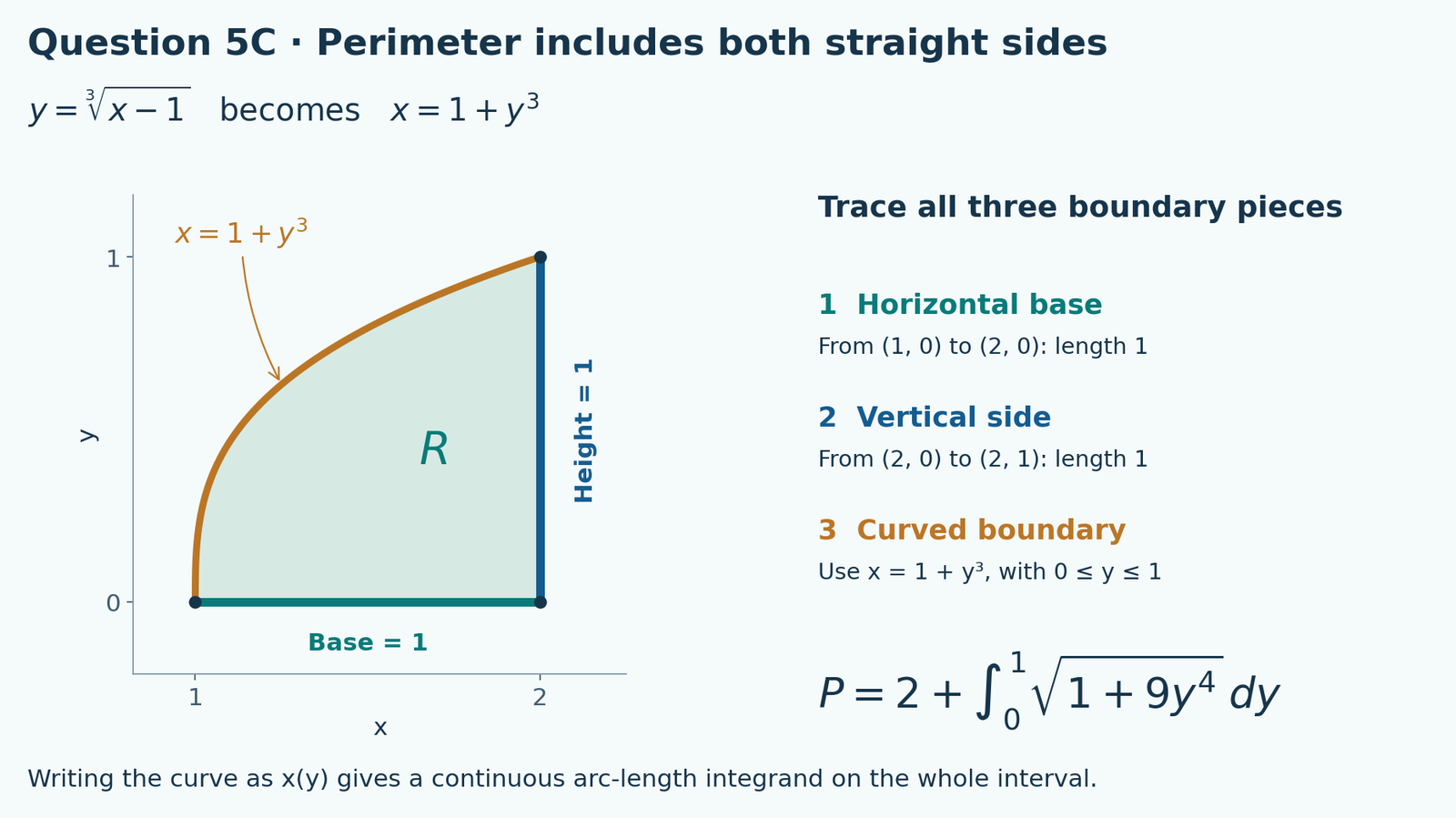
- The perimeter includes three pieces: the horizontal segment from to , the vertical segment from to , and the curve between and . The two straight segments have total length .
- Differentiate the curved boundary: for . Its arc length is .
- Thus . This is an improper arc-length integral at , understood as a right-hand limit.
- An equivalent expression avoids that endpoint singularity: solve for to obtain , with and . Therefore . Either expression gives the requested perimeter without evaluating it.
Credit check: Arc length uses , not . Include both straight boundary segments; the curved edge alone is not the perimeter.
Part D
- The upper limit is infinite, so begin with the definition of an improper integral: .
- The exponent has derivative , so an antiderivative is . Therefore .
- Evaluate at the finite endpoints: .
- As , . The limit exists and equals , so the improper integral converges.
Credit check: Use an explicit limit with a finite variable endpoint. Infinity is not a number to substitute into an antiderivative.
Maclaurin series and an alternating-series error bound
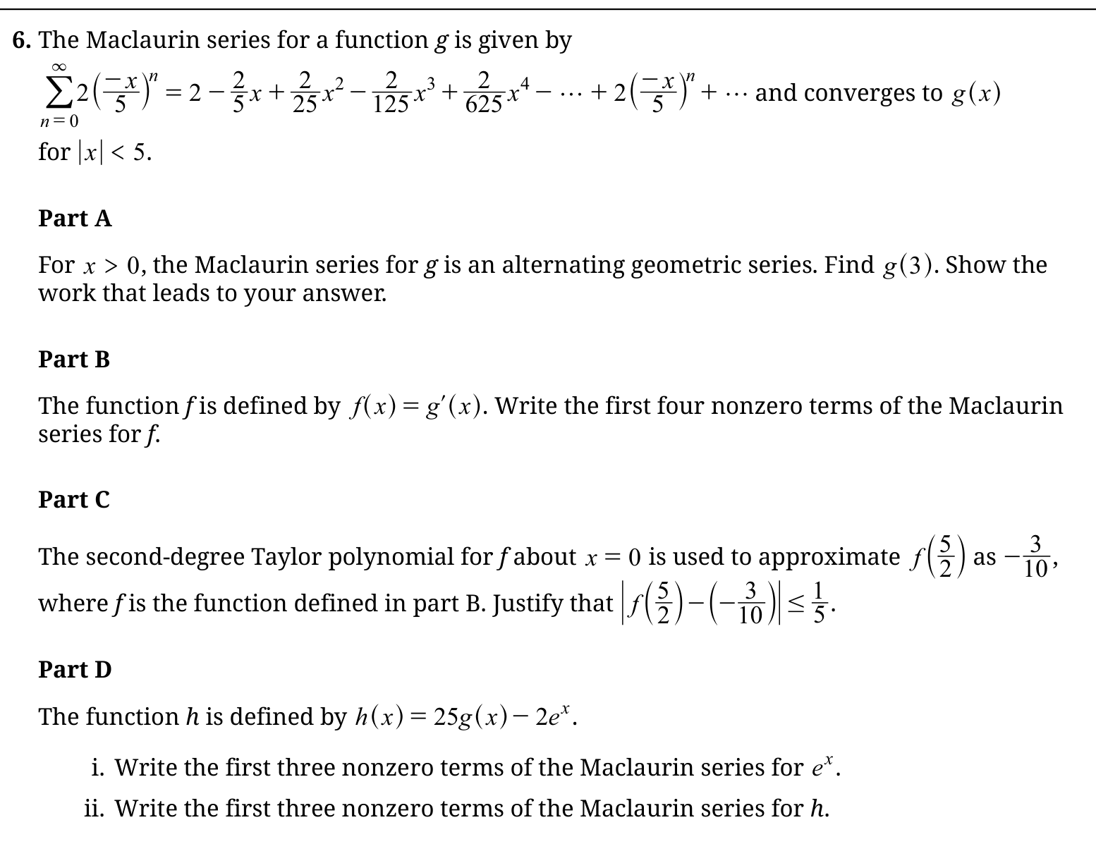
Part A
- At , the given series is geometric with first term and common ratio .
- Since , the infinite geometric sum exists and equals .
- Consequently .
Credit check: The ratio is negative. Subtracting it in the geometric-sum formula produces in the denominator.
Part B
- A power series may be differentiated term by term inside its interval of convergence. Here , so differentiate the given series for .
- The constant differentiates to zero. The next four terms give , , , and .
- Therefore for .
Credit check: Four nonzero terms of the derivative require looking through the term of the original series, because its constant term disappears.
Part C
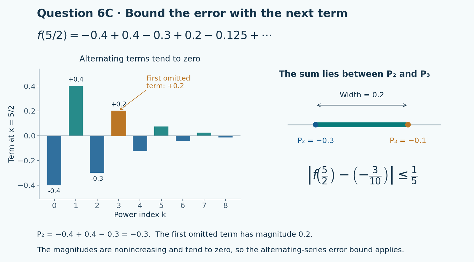
- From part B, the second-degree Taylor polynomial is . At it gives .
- At this positive input, the series for alternates in sign. Its term magnitudes, indexed from , are . They tend to zero and are nonincreasing; in fact, for . Thus the alternating series converges and satisfies the conditions for the Alternating Series Error Bound.
- The first omitted term after is the cubic term. Its magnitude at is .
- The absolute error is at most this magnitude: .
Credit check: Use the first omitted term and state why the alternating-series bound applies. The value is an upper bound for the error, not the error itself.
Part D(i)
- The Maclaurin series of the exponential function is .
- Take to obtain the first three nonzero terms: .
Credit check: The coefficients are reciprocal factorials: , , and .
Part D(ii)
- Use the original series for in the definition . Through degree two, .
- Scale the exponential series as well: .
- Subtract matching powers: . None of these three coefficients is zero.
Credit check: Distribute the minus sign across all terms of , and combine like powers before giving the answer.
Sources & References
Official question images: © 2026 College Board. Source pages are identified beneath each image. The solutions, explanatory diagrams, and feature artwork are original HeLovesMath materials. AP and Advanced Placement are registered trademarks of College Board. This page is not affiliated with or endorsed by College Board.
- College Board: AP Calculus BC past exam questions — the official release index, checked October 11, 2026.
- 2026 AP Calculus BC Free-Response Questions — 9-page released question PDF; Questions 1–6 appear on pages 3–4 and 6–9.
- 2026 AP Calculus BC Scoring Guidelines — 23-page official rubric used to check every subpart.
At the source check, the 2026 BC index listed one unnumbered free-response set and its scoring guidelines, with no separate 2026 question erratum linked. Course-and-exam-description updates for the 2026–27 school year are different documents and are not corrections to this released paper.